EXERCISE #1:
DIGITAL REPRESENTATION OF SIGNALS AND DIGITAL FREQUENCY ANALYSIS
Part A
Kyle M. White
Due: February 18, 2003
EEE 233: ADVANCED
DIGITAL SIGNAL PROCESSING
Department of
Electrical & Electronic Engineering
College of Engineering
& Computer Science
California State
University, Sacramento
Introduction
This project will explore various types of Fourier analysis available to engineers involved in digital signal processing. While the fundamental concept of Fourier series should be understood by the student in a graduate electrical engineering program, the details of the different types of analysis may be lacking. In this project we will use a non-periodic signal to explore the differences between the continuous Fourier transform, Fourier coefficients in a series expansion, and the DFT. This project is as much an exercise in using a computer to do these kinds of analyses as it is in the analyses themselves.
MATLAB is used extensively to generate plots for discussion and comparison. The code listing for the entire project is included in the appendix. The code is organized similar to the project in that one can follow the code from top to bottom in parallel with the discussion of the text. All of the graphs were made by putting a breakpoint at the appropriate point in the code to capture the plot. The interested reader can follow the discussion by referring to the code listing in the appendix.
Part 1 – Continuous Fourier transform
The signal in shown in Figure 1 will be used for the analysis. The input signal is a single rectangular pulse starting at time t = 0 with a duration of 0.025s and an amplitude of 750 (no units defined).
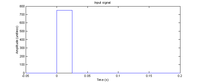
Figure 1 – MATLAB representation of the input signal
The input signal can be represented by a rectangle function of with delay of τ/2 and an amplitude A:
![]() (1)
(1)
Using a table of Fourier transforms and the time shifting property, we see that the continuous Fourier transform is:
![]() (2)
(2)
in terms of radian frequency, this is:
![]() (3)
(3)
It should be noted that in this project, the definition of the sinc function is:
![]()
Some texts define the sinc function differently.
MATLAB was used to create a representation of the Fourier transform of the aperiodic signal. See figure 2. This was done by plotting the Fourier transform function with a high enough resolution so that it looks continuous on the plot. The actual resolution used is .25 Hz in a range from –200 Hz to 200 Hz. This results in very smooth plots which accurately represent the continuous Fourier transform in both magnitude and phase. As expected, the zero-crossings occur every 1/τ because when f equals n/τ, sinc(πfτ) becomes sinc(πn) which is 0 for any integer n.
![]()
The phase plot is made by using the MATLAB angle function. This function wraps anytime the absolute value of the angle exceeds 2π. This is equivalent to the ‘unwrapped’ form and makes for an nice plot. These plots will be used as references for comparison in the following discussions.
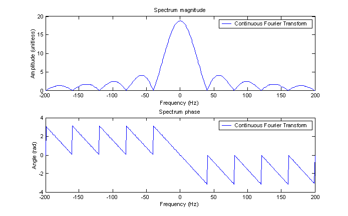
Figure 2 – MATLAB
representation of the Fourier transform of the input signal.
Part 2 – Fourier Series
The continuous Fourier transform is used to convert a continuous signal in the time domain into a continuous signal in the frequency domain. This is very nice for theoretical discussion where we can use continuous integrals but is impractical to use in real systems because we have neither an infinite amount of time nor an infinite amount of frequency to play with.
A more practical use of Fourier’s theory is the Fourier series. In this approach, a continuous time signal is measured continuously for a finite period of time Tg. The time Tg is commonly known as a gate or window of time in which the signal is measured. Using this approach, the Fourier transform can be found at discrete points. These points will be 1/Tg apart in the frequency domain. Thus, the larger Tg is, the more resolution will be gained in the Fourier series. This is a classic example of trade-off in engineering problems. To get more resolution, you need to sample for a longer period of time. To reconstruct the original signal from time 0 to Tg, the following relation is used:
 Where k
is an integer (4)
The series represents a set of sinusoids of frequency
2πkt/Tg and complex coefficient Xk that for any time
t = 0 to Tg, when added together, will reconstruct the original
signal at time t. The complex
coefficients Xk determine both the amplitude and phase of each
term. A side effect of this is that the
reconstructed signal will no longer be aperiodic. It will repeat every Tg.
The complex coefficients for our particular input signal given in equation (1) can be found in a table of Fourier series transforms combined with the time shifting property. This gives:
![]() (5)
(5)
Where fg = 1/Tg and k is any integer from -∞ to ∞. This is obviously very similar to the continuous Fourier transform for our input signal given in (2). In fact, equation (5) can be derived from (1) by substituting kfg for f and multiplying by 1/Tg. This suggests that the Fourier series represents the Fourier transform at specific points in the frequency domain kfg and scaled by 1/Tg.
Again, MATLAB was used to create and plot the coefficients, Xk, of the complex exponential Fourier series expansion of x(t) over the time 0 to 0.1 seconds. The result is shown in figure 3. We see that there is a point every 1/Tg or 10 Hz and that the zero crossing is every 40 Hz as we saw in the continuous plot.
The maximum value of the raw Fourier series is 187.5 which is 10 times the maximum value of the CFT. This makes sense because equation (5) has a factor of 1/Tg in the front which equation (2) does not have. This suggests that to achieve the same scale, we must multiply by the FS by a factor of Tg.
By scaling the Fourier series by Tg, and plotting it on the same graph as the continuous Fourier transform, we see that the Fourier series points exactly match the corresponding values of the Fourier transform in both magnitude and phase.
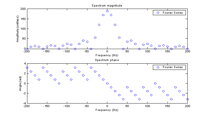
Figure 3 - Fourier series spectrum of the input signal
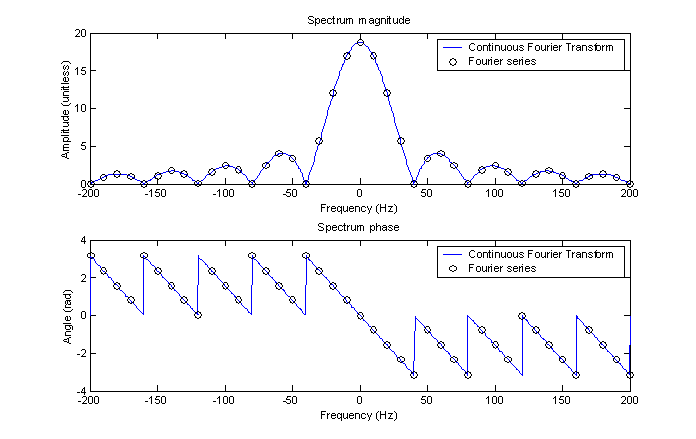
Figure 4 – Comparison plot of the continuous Fourier transform and Fourier series
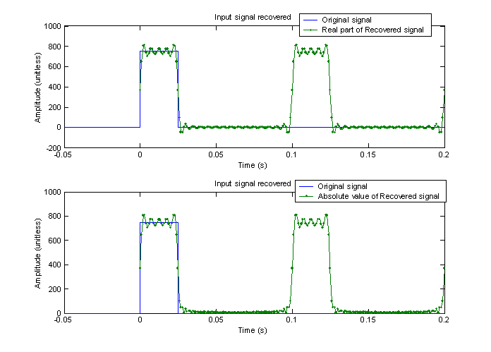
To see what happens when the signal is reconstructed, the coefficients that were found to create the plots in figure 3 were used to re-create the original signal using equation (4). Although the periodicity at Tg was expected, I was a bit confused on exactly how to produce the plot. After doing the summation as described in equation (4), the results in the time domain were still complex values. The imaginary components were small but not insignificant. This raises the question on how to plot. Should I just plot the real part or plot the absolute value? I chose to do both and compare. The result is shown in figure 5.
Figure 5 – Comparison of plotting the real part only vs. the absolute value of the recovered signal
In the real plot, there are some negative values especially near the transition points whereas these are smoothed out in the absolute value plot. In an actual DSP application, for this signal, either one could be used. I will leave future discussion of this point for later. Perhaps it will be explained in class or in part B or C of this project.
Part 3 – Discrete Fourier Transform (DFT).
While the Fourier series is pretty cool and certainly lends itself to implementing actual systems where we don’t have the luxury of infinite time, it still requires that we know the input signal continuously for the time 0 to Tg. This is often not the case when using computer systems to analyze and manipulate signals. A more realistic approach is to convert a sampled signal to the frequency domain
The DFT takes a set of discrete points in the time domain and transforms them into an equal number of discrete points in the frequency domain. Since both the time domain and frequency domain representation of the signal are discrete, the DFT is easily implemented in a digital computer. Additionally, if the number of samples is an integer power of 2 (e.g. 2,4,8,16,32 etc.) the DFT can be performed more efficiently in what is called the Fast Fourier Transform. MATLAB has a function fft which performs the FFT when possible (number of samples = 2n) and does a DFT otherwise.
For this project, a 32 point FFT is performed with the MATLAB fft function. Figure 6 shows the sampled input signal compared to the continuous input signal.
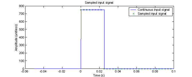
Figure 6 – 32 point sampled input signal
The output of the fft function is a symmetrical matrix about the halfway point of the number of points used in the FFT. This is a by-product of the DFT algorithm used and is easily fixed in MATLAB with the fftshift function.
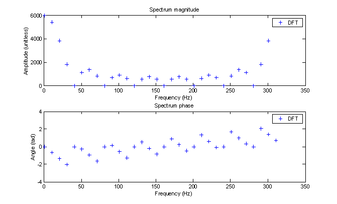
Figure 7 – Raw 32 point FFT
The maximum amplitude of the raw FFT is 6000. The maximum amplitude of the continuous Fourier transform is 18.75. Thus, to get the proper scaling factor, we divide 18.75 by 6000 to get 1/320. I suspect 320 comes from 10 times 32 which is 1/ Tg times the number of points N of the FFT. To get the same scale as the raw FS, we would need to divide by 32 which is N. These scale factors are summarized in table 1. To use the table, start with what you have in the row, then find what you want in the column. Use the value at the intersection as the scale factor to convert.
Table 1 – Scale
factors for converting between different Fourier transforms
|
|
CFT |
FS |
DFT |
|
CFT |
1 |
1/Tg |
N/Tg |
|
FS |
Tg |
1 |
N |
|
DFT |
Tg/N |
1/N |
1 |
After shifting and scaling, the FFT is plotted on top of the continuous Fourier transform and Fourier series for comparison in figure 8.
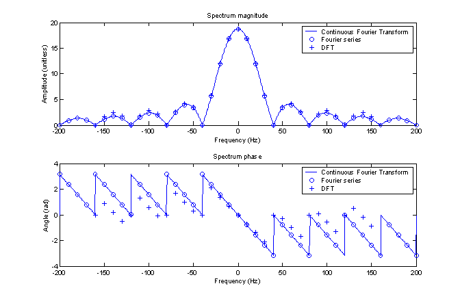
Figure 8 –
Comparison of continuous Fourier transform, Fourier series and DFT
As expected, the DFT (or FFT) does not exactly correspond to the Fourier transform or Fourier series, especially as the absolute value of the frequency goes up. To illustrate, a vector was created in MATLAB of the normalized error using
![]()
Using the eyeball method and the fact that the magnitude spectrum is symmetrical, I determined that a quadratic fit might illustrate how the error increases as a function of frequency. To get it right, the first point had to be dropped since the 32 points include the center at a frequency 0, therefore the total number of points has to be odd in order to be symmetrical. Also, the zero-crossing points were dropped as they caused divide by 0 problems and clearly didn’t represent the general trend of the error. The result of the magnitude error along with a quadratic curve fit is shown in figure 9. MATLAB makes it very easy to check out different types of best fit curves but all that was needed was a simple quadratic.
Seeing a parabola in the frequency domain that represents error reminds me of the power spectral density of noise in an FM receiver. In demodulating FM, the further away from the carrier frequency you get, the more noise is introduced which is why FM stereo is more difficult to pick up than mono. I’m not sure how that is related to the results found here but I’ll bet there is a relation.
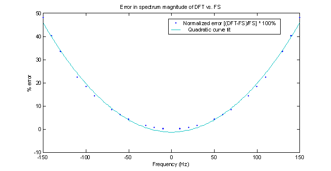
Figure 9 –
Normalized magnitude error of the DFT vs. FS with a quadratic best fit curve
A similar method was used to analyze the error of the phase. The value of the phase, however, is a pure number (radians) and therefore does not need to be normalized. Simply taking the difference between the FS and DFT and removing the same zero-crossing points results in a linear relationship between the phase error and frequency. This is shown in figure 10.
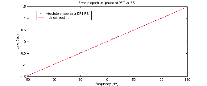
Figure 10 –
Absolute error in phase of DFT compared to FS (no zero points)
In order to perform a DFT with more than 32 points one must consider where the points will come from. There are clearly two choices here. First, we could use the same time window and just sample the input function at a higher resolution, that is, with a smaller ∆t. This will result in a DFT with more output points (same as the input) with the same spacing in the frequency domain 1/Tg. Thus the extra points must describe higher frequencies (both positive and negative). Another way to go would be to keep ∆t the same and make the time window bigger by padding the function with extra zeros. In this scenario, the total frequency range of the output will remain the same but the resolution in the frequency domain will increase because the spacing is 1/Tg. Once again, as the sample time is increased, so is the resolution in the frequency domain. The second option is demonstrated here.
In order to continue using the FFT as opposed to the DFT, the total number of points N must remain an integer power of 2. It was increased by a factor of 4 to 128. Figure 11 was created exactly as figure 8 but with a 128 point FFT instead of a 32 point. As can easily be seen, the range of frequencies is the same but the resolution has greatly increased (by a factor of 4 I’d say). As before, the scale factor needed to compare with the CFT was Tg/N where Tg = 0.4 and N = 128. 0.4/128 = 1/320 = 0.003125 which is ∆t. The errors appear to be following the same pattern as before but analyses was not done.
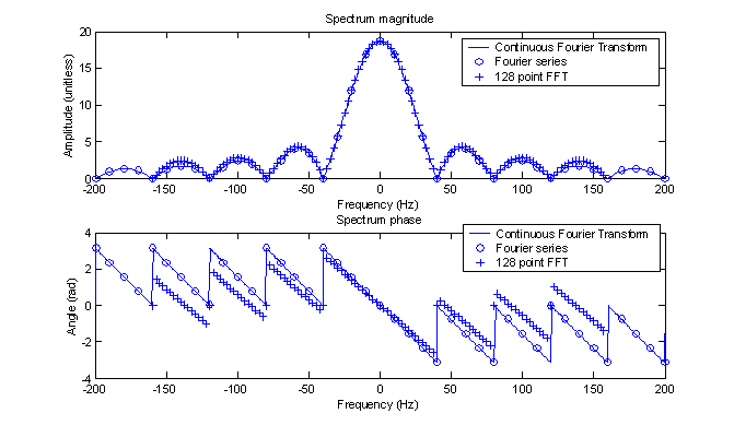
Figure 11 –
Comparison of the Fourier transforms using a 128 point FFT.
Conclusion
In part A, three types of Fourier transforms were performed on a single aperiodic input signal and compared to each other. It was found that the Fourier series exactly represents the continuous Fourier transform at specific frequencies. It was also found that the DFT (or FFT) also represents the continuous Fourier transform at specific frequencies but that it has an error which increases quadratically in magnitude and linearly in phase as the frequency increases for the given input function. I suspect that this is not true for all input functions, otherwise it would be trivial to come up with a correction scheme and we would all be using it.
This project has made very clear the differences and
similarities of the three types of transforms studies. It has also demonstrated
the use of computer software to do Fourier analysis.
Appendix – Code listing for the entire project
% Kyle M.
White
% EEE 233
Advanced DSP
% Exercise
#1: Digital representation of signals and digital frequency analysis
% Part A -
Compare the continuous Fourier transform, Fourier series and DFT
clear;
A = 750;
tau =
.025; % seconds
% Plot an
approximation of the input signal. For display only.
t1 = [-.05 0
.0001 .02499 .02501 .2];
xt1 = [0 0 1
1 0 0];
xt1 = A*xt1;
plot(t1,xt1,'-');
title('Input
signal');
xlabel('Time
(s)');
ylabel('Amplitude
(unitless)');
% Plot the
continuous Fourier transform
range =
200; % chosen because it
results in a nice plot.
step =
.25; % This determines
the resolution
f1 =
-range:step:range; % Frequency in Hz
from -range Hz to range Hz with a resolution of 1 Hz
w =
2*pi*f1; % Frequency in
radians
Samples =
(2*range/step)+1; % Number of samples created, this will be used for the max
array index
for i =
1:Samples;
Xw(i) =
A*tau*(ksinc(tau*w(i)/2))*exp(-j*tau*w(i)/2);
end
subplot(2,1,1);
plot(f1,abs(Xw));
title('Spectrum
magnitude');
xlabel('Frequency
(Hz)');
ylabel('Amplitude
(unitless)');
legend('Continuous
Fourier Transform');
subplot(2,1,2);
plot(f1,angle(Xw));
title('Spectrum
phase');
xlabel('Frequency
(Hz)');
ylabel('Angle
(rad)');
legend('Continuous
Fourier Transform');
% Plot the
Fourier series using a time gate Tg
subplot(1,1,1);
Tg = .1; % seconds
fg =
1/Tg; % Hz
wg =
2*pi*fg; % radians
% Create a
range that will be the same as above. Try to get 5 humps on each side (fmax =
200Hz)
range =
5*Tg/tau;
k =
-range:1:range;
Samples =
2*range+1;
for i =
1:Samples;
f2(i) = k(i)*fg;
Xk(i) =
(A*tau/Tg)*ksinc(tau*k(i)*wg/2)*exp(-j*tau*k(i)*wg/2);
end
% Do the plot
subplot(2,1,1);
plot(f2,abs(Xk),'o');
title('Spectrum
magnitude');
xlabel('Frequency
(Hz)');
ylabel('Amplitude
(unitless)');
legend('Fourier
Series');
subplot(2,1,2);
plot(f2,angle(Xk),'o');
title('Spectrum
phase');
xlabel('Frequency
(Hz)');
ylabel('Angle
(rad)');
legend('Fourier
Series');
% Scale by Tg
Xk = Xk*Tg;
% Do the
comparison plot
subplot(2,1,1);
plot(f1,abs(Xw),'-',f2,abs(Xk),'ok');
title('Spectrum
magnitude');
xlabel('Frequency
(Hz)');
ylabel('Amplitude
(unitless)');
legend('Continuous
Fourier Transform','Fourier series');
subplot(2,1,2);
plot(f1,angle(Xw),'-',f2,angle(Xk),'ok');
title('Spectrum
phase');
xlabel('Frequency
(Hz)');
ylabel('Angle
(rad)');
legend('Continuous
Fourier Transform','Fourier series');
% Recover the
input signal from Fourier series
% Unscale Xk
Xk = Xk/Tg;
kmax = 20;
trange = .2;
tstep = .001;
t =
0:tstep:trange;
tSamples =
(trange/tstep)+1;
for tindex =
1:tSamples;
xrec(tindex) = 0;
for i = 1:2*kmax +1; % For all the Xks that we
have
xrec(tindex) = xrec(tindex) + Xk(i)*exp(j*k(i)*2*pi*t(tindex)/Tg);
end
end
subplot(2,1,1);
plot(t1,xt1,'-',t,real(xrec),'.-');
title('Input
signal recovered');
xlabel('Time
(s)');
ylabel('Amplitude
(unitless)');
legend('Original
signal','Real part of Recovered signal');
subplot(2,1,2);
plot(t1,xt1,'-',t,abs(xrec),'.-');
title('Input
signal recovered');
xlabel('Time
(s)');
ylabel('Amplitude
(unitless)');
legend('Original
signal','Absolute value of Recovered signal');
% Do the FFT
% create the
sample index
% fs = 320Hz
T=.1s
Samples = 32;
T = .1;
Step =
T/Samples;
% The sampled
signal and n
for i =
1:Samples;
n(i) = i - 1;
ndt(i) = n(i)*Step;
if ndt(i) < tau
xn(i) = A;
else
xn(i) = 0;
end
end
% Change the
range of the original signal for a better plot
t1 = [-.05 0
.0001 .02499 .02501 .1];
% Plot the
sampled input signal vs. the continuous signal
subplot(1,1,1);
plot(t1,xt1,'-',ndt,xn,'x');
title('Sampled
input signal');
xlabel('Time
(s)');
ylabel('Amplitude
(unitless)');
legend('Continuous
input signal','Sampled input signal');
X = fft(xn);
maxf =
(1/T)*(Samples);
f =
1:1/T:maxf;
% Plot the
raw DFT
subplot(2,1,1);
plot(f,abs(X),'+');
title('Spectrum
magnitude');
xlabel('Frequency
(Hz)');
ylabel('Amplitude
(unitless)');
legend('DFT');
subplot(2,1,2);
plot(f,angle(X),'+');
title('Spectrum
phase');
xlabel('Frequency
(Hz)');
ylabel('Angle
(rad)');
legend('DFT');
% Fix the DFT
so it looks normal
% Scale and
shift
Xn =
fftshift(X)*T/Samples;
% Shift the
frequency
for i = 1:32
ft(i) = f(i) - (maxf+2)/2;
end
% re-scale Xk
by Tg
Xk = Xk*Tg;
% Do the
comparison plot
subplot(2,1,1);
plot(f1,abs(Xw),f2,abs(Xk),'ob',ft,abs(Xn),'+b');
title('Spectrum
magnitude');
xlabel('Frequency
(Hz)');
ylabel('Amplitude
(unitless)');
legend('Continuous
Fourier Transform','Fourier series','DFT');
subplot(2,1,2);
plot(f1,angle(Xw),f2,angle(Xk),'ob',ft,angle(Xn),'+b');
title('Spectrum
phase');
xlabel('Frequency
(Hz)');
ylabel('Angle
(rad)');
legend('Continuous
Fourier Transform','Fourier series','DFT');
% Find the
differences between the Fourier series and DFT
% Trim the
Fourier series vector to be the same size as the DFT
Start = 5
x = 1;
for i =
Start:Start+31;
Xktrim(x) = Xk(i);
fc(x) = f2(i);
x = x+1;
end
FS = Xktrim;
DFT = Xn;
AbsXn =
abs(Xn);
PhXn = angle(Xn);
AbsXktrim =
abs(Xktrim);
PhXktrim =
angle(Xktrim);
for i = 1 :
32;
DeltaMag(i) = 100*(AbsXn(i) -
AbsXktrim(i))/AbsXktrim(i);
%DeltaPhase(i) = (((angle(Xn(i)) -
angle(Xktrim(i)))/angle(Xktrim(i)))*100);
NormalizedErrorMag(i) = 100*(abs(DFT(i)) -
abs(FS(i)))/abs(FS(i));
NormalizedErrorPhase(i) = (angle(DFT(i)) -
angle(FS(i))); %)/angle(FS(i));
end
% Get rid of
first point to make symmetrical
DeltaMadFix =
DeltaMag(2:32);
NormalizedErrorMagSym
= NormalizedErrorMag(2:32);
NormalizedErrorPhaseSym
= NormalizedErrorPhase(2:32);
fc =
fc(2:32);
% strip the
zeros
x = 1;
for i = 1:31;
if NormalizedErrorMagSym(i) > .01
NormalizedErrorMagSymNoZeros(x) =
NormalizedErrorMagSym(i);
NormalizedErrorPhaseSymNoZeros(x) =
NormalizedErrorPhaseSym(i);
fcNoZeros(x) = fc(i);
x = x +1;
end
end
%NormalizedErrorPhaseSymNoZeros
= NormalizedErrorPhaseSym;
% Plot the
difference vectors
subplot(1,1,1);
plot(fcNoZeros,NormalizedErrorMagSymNoZeros,'.');
title('Error
in spectrum magnitude of DFT vs. FS');
xlabel('Frequency
(Hz)');
ylabel('%
error');
legend('Normalized
error [(DFT-FS)/FS] * 100%');
%subplot(1,1,1);
plot(fcNoZeros,NormalizedErrorPhaseSymNoZeros,'.');
title('Error
in spectrum phase of DFT vs. FS');
xlabel('Frequency
(Hz)');
ylabel('Error
(rad)');
legend('Absolute
phase error DFT-FS');
% Do the FFT
% create the
sample index
% fs = 320Hz
T=3.2s
Samples =
128;
T = .4;
Step =
T/Samples;
% The sampled
signal and n
for i =
1:Samples;
n(i) = i - 1;
ndt(i) = n(i)*Step;
if ndt(i) < tau
xn(i) = A;
else
xn(i) = 0;
end
end
X = fft(xn);
maxf =
(1/T)*(Samples);
f =
1:1/T:maxf;
% Plot the
raw DFT
subplot(2,1,1);
plot(f,abs(X),'+');
title('Spectrum
magnitude');
xlabel('Frequency
(Hz)');
ylabel('Amplitude
(unitless)');
legend('DFT');
subplot(2,1,2);
plot(f,angle(X),'+');
title('Spectrum
phase');
xlabel('Frequency
(Hz)');
ylabel('Angle
(rad)');
legend('DFT');
% Fix the DFT
so it looks normal
% Scale and
shift
Xn =
fftshift(X)*T/Samples;
% Shift the
frequency
for i =
1:Samples
ft(i) = f(i) - (maxf+2)/2;
end
% Do the
comparison plot
subplot(2,1,1);
plot(f1,abs(Xw),f2,abs(Xk),'ob',ft,abs(Xn),'+b');
title('Spectrum
magnitude');
xlabel('Frequency
(Hz)');
ylabel('Amplitude
(unitless)');
legend('Continuous
Fourier Transform','Fourier series','128 point FFT');
subplot(2,1,2);
plot(f1,angle(Xw),f2,angle(Xk),'ob',ft,angle(Xn),'+b');
title('Spectrum
phase');
xlabel('Frequency
(Hz)');
ylabel('Angle
(rad)');
legend('Continuous Fourier Transform','Fourier series','128 point FFT');
