EXERCISE #1:

 

DIGITAL REPRESENTATION OF SIGNALS AND DIGITAL FREQUENCY ANALYSIS

 

Parts B, C and D

 

 

 

 

Kyle M. White

 

Due: Tuesday, March 11, 2003

 

 

 

 

 

 

 

 

 

EEE 233: ADVANCED DIGITAL SIGNAL PROCESSING

 

Department of Electrical & Electronic Engineering

College of Engineering & Computer Science

California State University, Sacramento

Introduction

In part A of this exercise three types of Fourier analyses on an aperiodic function were explored.  The continuous Fourier transform (CFT), Fourier series (FS) and discrete Fourier transform (DFT) were all calculated, evaluated and plotted for comparison.  It was determined that the Fourier series represented the CFT at discrete points in the frequency domain while the DFT gave approximations to those points with an error that increased with the frequency.

 

In part B, similar analyses are done for a periodic cosine function.  Also, different types of windowing will be explored with the DFT to see how well each performs in giving an accurate representation of the CFT.  Part C will explore the effects of quantization of the input signal and in part D the frequency of the input signal will be increased to demonstrate the effects of aliasing. For these parts, only the magnitude will be analyzed as the phase is zero for our input signal.

 

As in part A, MATLAB is used extensively to generate plots for discussion and comparison.  The code listing for the entire project is included in the appendix. The code is organized similar to the project in that one can follow the code from top to bottom in parallel with the discussion of the text. All of the graphs were made by putting a breakpoint at the appropriate point in the code to capture the plot and in some cases, text and arrows were added directly to the plot. The interested reader can follow the discussion by referring to the code listing in the appendix.

Part B – Fourier analysis of a sinusoid

 

B1 - Continuous Fourier transform (CFT)

 

The signal in shown in Figure 1 is used for the analysis.  The input signal is a simple cosine function with a frequency of 35 Hz, no phase shift and an amplitude of 750 (no units defined).

 

                                                                                              where ω₀ = 2π(35 Hz), A = 750

 

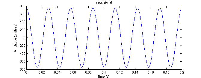
Figure 1 – MATLAB representation of the input signal

 

This is perhaps the most elementary function for doing Fourier analyses. The continuous Fourier transform is found in any table of Fourier transforms and is:

 

                                                                                                   (1)

 

This is represented graphically as two δ functions at ± ω₀ with coefficients Aπ as shown in figure 2. 

 

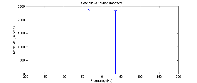
Figure 2 – MATLAB representation of the Fourier transform of the input signal.

 

Although the vertical scale on the plot accurately represents the coefficients in front of the δ functions (representing the area under the curve), the two lines of spectra have an infinite magnitude and infinitely small width, as indicated by the arrows. The δ functions present a problem when trying to compare the amplitude of the CFT with the amplitudes of the Fourier series and DFT.  In order to provide some means of comparison, the δ function can be approximated with a pulse of duration є and amplitude 1/є.  The choice of є is arbitrary but by choosing є to be 2π radians (1 Hz), the amplitude of the CFT becomes A/2 which will coincide very nicely with both the Fourier series and the DFT (when enough points are used).

 

With this approximation, the CFT appears as in figure 3.

 

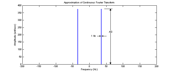
Figure 3 – Approximation of δ functions with є = 2π  = 1 Hz

 

B2 – Fourier Series (FS)

 

As in part A, Fourier series analysis is done with a time gate T_g = 0.1 seconds.  This leads to the following equation which represents the Fourier series coefficient X_kg using a time gate T_g of a cosine with frequency ω₀ and no phase shift:

 

                                (2)

 

Figure 4 shows the plot of the magnitude of the coefficients along with the CFT approximation from figure 3.  Since the time gate Tg is not an integer multiple of the period of the cosine function, there does not exist a spectral line at the frequency ω₀.  The spectral lines appear at n/Tg which is ±10, ±20, ±30 Hz etc. This is an example of the worst case scenario when using a finite time gate to do a Fourier series on an input signal with a known frequency.

 

Unlike the results found in part A, the Fourier series for this input signal does not represent the CFT at discrete frequencies for the input function.  In fact, we know that the only frequency that really exists is 35 Hz yet that particular frequency is missing from the Fourier series and there are a whole bunch of frequencies in the Fourier series which do not exist in the original function.  The ‘real’ frequency lies halfway between the two highest coefficients indicating that at least the series is close. For this input function, no scaling was needed to compare with the approximated CFT. 

 

This happens because in part A the time gate Tg included the entire signal with some zero padding whereas with a periodic function such as the cosine, we are ‘chopping off’ most of the function by choosing Tg and repeating that portion every Tg.  What we are seeing is discrete points of the continuous Fourier transform in the frequency domain of a cosine function seen through a window between t = 0 and 0.1 seconds.

 

 

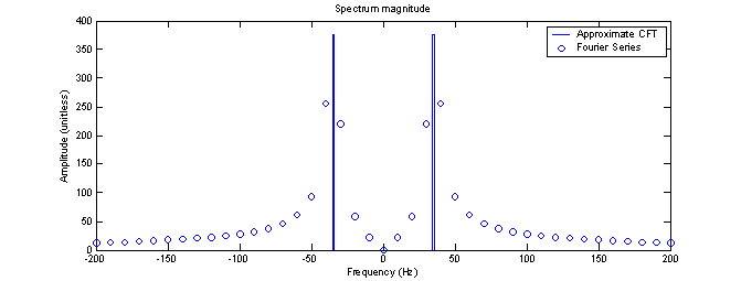
Figure 4 – Fourier series with time gate Tg = 0.1s

 

This windows happens to be a rectangular window but, as we will see in the DFT section, windows of other shapes can be used which yield much different results.  The rectangular window and the resulting function that this Fourier series really represents is shown in figure 5. The sharp points seen at Tg cause all kinds of high frequency components to be included.  Now, had Tg been chosen to be an integer multiple of f₀, then there would be no sharp points and therefore no high frequency components.

 

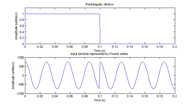
Figure 5 – Rectangular window (no padding) and the effect it has on the input function

 

B3 – Discrete Fourier  Transform (DFT)

 

As always, in order to perform a DFT, the input signal must be sampled at a finite frequency for a finite period of time.  The sampled input is shown in figure 6. As can easily be seen, there are well over two points sampled for every period, therefore the Nyquist sampling rate is satisfied and there should be no aliasing indicated in the frequency domain.  In the aliasing section, we will see what happens when this is not the case.

 

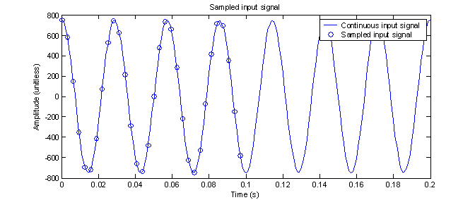
Figure 6 - Sampling of the input function for a 32 point DFT

 

Figure 7 shows the output of the 32 point DFT after shifting and scaling by 1/N along with the CFT and Fourier series.  Again, no scaling by Tg was necessary.  As in part A, the DFT looks very much like the FS.  As opposed to the results in part A, this time the error between the FS and DFT is not less at the lower frequencies.  In fact, the DFT shows a significant DC component whereas the FS correctly shows no DC component. 

 

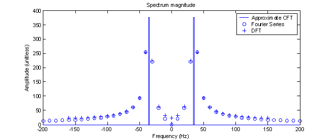
Figure 7 – Comparison of the CFT, FS, and DFT

B4 – Padding and windowing

 

One way to improve the results of the DFT is, of course, to add more points. As in part A, this was done by zero padding the rectangularly windowed input function.  This time, however, a 1024 point FFT was done to show smooth lines on the plots.  The result is shown in figure 8.  Since we now have such a ‘high’ resolution in the frequency domain, this plot is shown with connecting lines and we see that the points obtained with the Fourier series and 32 point DFT were really just (mostly) the peaks of a sinc function and not part of a smooth curve representing the envelope of the peaks as one might have assumed.  This illustrates how one can be fooled by a spectrum with a limited resolution.  For the 1024 DFT, the main lobes reach a maximum width of 20 Hz before the function begins to ascend.  The maximum side lobe is 94.3/375.5 or 25% of the main lobe.

 

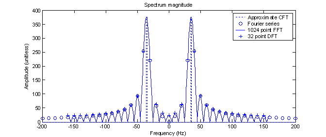
Figure 8 – Comparison 1024 Point FFT with 0 padding to previous transforms

 

Notice that the points from the 32 point DFT correspond exactly with the line obtained with the 1024 point DFT.

 

In order to compare the padded 1024 DFT with the other transforms, a scale factor of 1/32 was used.  This is not 1/N (the number of samples) as N has been increased to 1024.  I call this 1/N_win because it’s one over the number of points used in the window.  As discovered in part A, when doing a DFT, the transform must scaled by 1/N to get the DFT results to be comparable in amplitude with the Fourier series and CFT.  When padding a truly periodic signal, however, the power of the signal for the total number sample time NΔt is effectively reduced to N_win/N and this transfers to the frequency domain when doing the DFT.  In order to make up for this loss, the transform needs to then be multiplied by N/N_win (in addition to the normal multiplication of 1/N).  The Ns cancel and we are left with just 1/N_win.

 

The scale factors are summarized in table 1.  To use the table, start with what you have in the row, then find what you want in the column. Use the value at the intersection as the scale factor to convert.  In contrast to part A, there are no Tg factors in the table and there is an extra row and column for the padded DFT.  The fact that there are no Tg factors in the table as in part A is due to the choice of є in determining the approximation of the CFT.  As stated before, this is an arbitrary choice and I could have easily chosen something like 1Hz/Tg which would make the CFT approximation shorter and fatter.  Its amplitude would then be ATg/2 = 37.5. If that were the case, then the other transforms would also need to be multiplied by Tg to be comparable with the CFT and Table 1 would look very much like Table 1 in part A

 

Table 1 – Scale factors for converting between different Fourier transforms.

 

 

Another way to potentially improve the spectrum is to use a window other than a rectangle.  Unless the sample period is an integer multiple of one of the prominent frequencies in the input signal, a rectangular window almost guarantees sharp transitions which lead to high frequency components.  By multiplying the input signal by a window function which gradually goes to zero at both ends, the sharp transitions are eliminated.  One such window is the triangle window shown in figure 9.

 

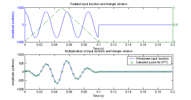
Figure 9 – Zero padded input function with a triangular window

 

Figure 9 shows the triangle window and its effect on the input signal along with the samples used for the following DFT (showing only 64 of the samples).  It’s easy to see how the window smoothes out the function at the edge of the window.  This should result in fewer high frequency components in the frequency domain (side lobes).

 

Figure 10 shows the magnitude spectrum after doing the DFT.  The results here show much lower side-lobes but wider main lobes.  The main lobes reach a maximum width of 37 Hz before the function begins to ascend.  The largest side lobe has an amplitude of 9/186.4 or 4.8% of the main lobe.

 

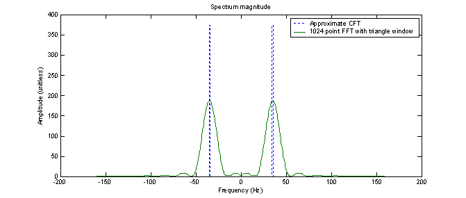
Figure 10 – 1024 point FFT with triangle window.

 

There are many different types of windows that can be used to modify the input function before performing the DFT. Several of these are shown in the time domain in figure 11.

 

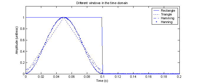
Figure 11 – Comparison of four different window functions in the time domain.

 

The areas under the curves of the non-rectangle window functions are much less than the area under the rectangle function.  This means that, when multiplied by the window function, the input function will lose much of its power.  That is, the absolute value of the area under the square of the modified function will be much less than it was before the window modification.  This is seen in both figures 10 and 12 (DFT of the windowed functions) as they all have much less areas under their curves than the DFT of the non-windowed function.

 

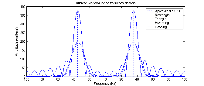
Figure 12 – Comparison of four differently windowed functions in the frequency domain.

 

Figure 13 shows a close-up of the transition point from the main lobes to the side lobes of all the windows and thus gives a better indication of how the different windows behave.

 

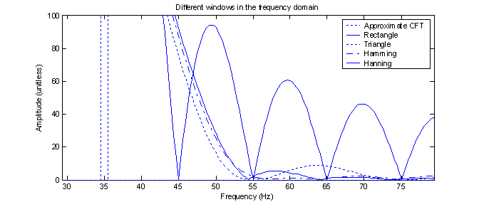
Figure 13 – Close up of figure 12

 

Each window has its own unique properties.  From figure 13, it is clear that the Hamming window has the flattest response after about 55 Hz.  The rectangle window has by far (10 Hz), the narrowest main lobe.  The triangle and Hanning windows seem to both be compromises between these two extremes.  There is no ‘best’ window, just different windows.  If there was a best window, we’d probably only learn about that one and not even bother with the others.

 

Part C – Quantization

 

One usually studies DSP in hopes of learning to process analog signals with a digital computer.  Sampling, however, is only half the story when it comes to converting an analog signal to digital. The other half of the story is called quantization and it, of course, adds more errors.  ‘But we have been doing Fourier transforms with a digital computer already’ one might say.  True, but these values were calculated, not measured and, thus far, the quantization has been to the limits of the software which uses 64 bits to represent a floating point number.  Therefore the number of quantization levels has been 2⁶⁴ or roughly 18 x 10¹⁸.  This resolution is so high it is not much of an issue, especially when doing DFTs on the order of 1024 points.  To simulate a more realistic system, the quantization level should be much lower.

 

To quantize the input cosine function, a 3 bit (8-level) quantizer was created with the aid of the MATLAB uencode function.  The quantized signal is shown in figure 14 along with the quantization error.

 

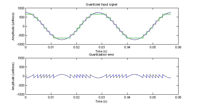
Figure 14 – 8 level quantization of the input signal over two periods

 

 

To calculate the amount of error (or noise) introduced by quantization, we can compare the RMS values of the original signal and the error signal.  A sinusoidal signal has a theoretical RMS value of  which comes out to be 530.3301.  By summing the squares of the elements in the vector used to create figure 14 and taking the square root, the RMS is calculated to be 530.3632…. pretty close.  This indicates that the method used in MATLAB is accurate. By applying the same method to the quantization error vector, its RMS is calculated to be 58.8714.  Thus the %RMS error of the quantized signal is

 

 

An often used measure of error (or noise) is the signal to noise ratio or SNR usually expressed in dB.  For uniform quantization, a common formula used to find the SNR of the input signal to quantization noise is:

 

                            where n = number of bits

 

In this case, with 3 bit quantization, it turns out to be 10.76 dB.

 

To see what happens when we take the DFT of a quantized signal, a 128 point FFT was performed.  The result is shown in figure 15.

 

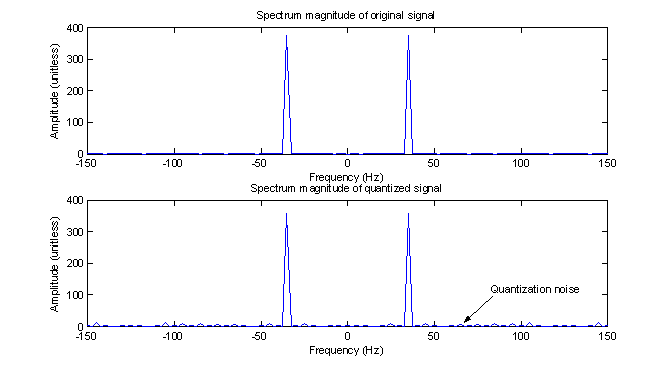
Figure 15 – Comparison of 128 FFT of original and quantized signals

 

Figure 15 illustrates two ideas.  First, by taking a 128 point FFT without padding, that is, using the original signal for the entire sample period instead of using zeros, we get a spectrum which looks much more like the ideal CFT (with the main lobe amplitude of A/2).  Secondly, the FFT of the quantized signal shows noise at many frequencies whereas in the original signal, the noise is barely noticeable.

 

Part D – Aliasing

 

So far, Nyquist sampling rate has been obeyed by choosing a sample rate of 320 Hz while the maximum frequency component of the desired signal remained at 35 Hz.  To see what happens when the Nyquist rate is violated, the frequency on the input signal is increased past ½ of the sample rate.  Figure 16 shows the results of four different signal frequencies (100, 200, 320 and 350 Hz) in both the time domain and frequency domain.  One can see that as soon as the frequency of the signal exceeds ½ the sample rate F_s = 320 Hz, the resulting signal no longer represents the original signal.  It now represents an alias signal at frequency F_s – F_o.

 

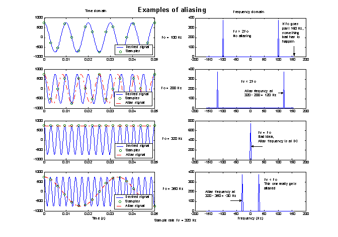
Figure 16 – Aliasing in the time domain and frequency domain

 

Conclusions

 

As always for these kinds of projects, many questions were answered.  This project made it clear that it’s impossible to use a computer to calculate exactly the continuous Fourier transform as there is no way to calculate infinity.  You can get a good representation though if you sample with enough points.  Even 128 points does a pretty good job when those points are all taken from the signal (as opposed to padding). The exercise also demonstrated the differences between doing Fourier analysis on a periodic vs. an aperiodic signal.  The effects of padding and windowing were seen and compared and it was made clear that both make a big difference.  Which one is preferred, however, is still a question that can only be answered for a particular application.

 

Part C demonstrated the effect of quantization noise and part D clearly shows the how aliasing can occur if the Nyquist rate is not met.  As in part A, much was learned about MATLAB and programming in general for Fourier analysis, which is of course, the ultimate goal in learning DSP.

Appendix – Code listing for parts B, C and D

 

% Kyle M. White

% EEE 233 Advanced DSP

% Exercise #1: Digital representation of signals and digital frequency analysis

% Part B, C and D

clear;

A = 750;

fo = 35;        % Frequency of the input sinusoid

tau = .025;     % seconds

%MaxFreq = 100;  % Hz - Used for all graphs. Must be > fo

TwoPi = 2*pi;   % Just because it's used a lot, no need to re-compute everytime

 

% ============ Plot an approximation of the input signal. For display only. =============

 

t1 = 0:.001:.2;

xt1 = A*cos(TwoPi*fo*t1);

plot(t1,xt1,'-');

title('Input signal');

xlabel('Time (s)');

ylabel('Amplitude (unitless)');

 

% ============ Create a representation of the continuous Fourier transform ============

Tg = .1;          % seconds

MaxFreq = 200;

f1 = [-MaxFreq -fo 0 fo MaxFreq];

Xf1 = pi*A*[NaN 1 NaN 1 NaN];

stem(f1,Xf1,'^');

title('Continuous Fourier Transform');

xlabel('Frequency (Hz)');

ylabel('Amplitude (unitless)');

 

% Create a representation of the approximation of the continuous Fourier transform

DelF = 1; % Hz = 2*pi radians ; %1/Tg;

LittleTeenyBit = .00001;

MaxFreq = 200;

f1 = [-MaxFreq -fo-DelF/2 -fo-DelF/2+LittleTeenyBit -fo+DelF/2 -fo+DelF/2+LittleTeenyBit fo-DelF/2 fo-DelF/2+LittleTeenyBit fo+DelF/2 fo+DelF/2+LittleTeenyBit MaxFreq];

Xf1 = (A/2)*[0 0 1 1 0 0 1 1 0 0];

plot(f1,Xf1,'-');         

title('Approximation of Continuous Fourier Transform');

xlabel('Frequency (Hz)');

ylabel('Amplitude (unitless)');

 

% ============ Plot the Fourier series using a time gate Tg = 0.1 ============

Tg = .1;          % seconds

fg = 1/Tg;        % Hz

wg = TwoPi*fg;    % radians

wo = TwoPi*fo;    % radians

 

% Create a range that will be the same as above. fmax = 200Hz

range = 20;

Samples = 2*range + 1;

k = -range:1:range;

% Calculate the Fourier series

for i = 1:Samples;

    f2(i) = k(i)*fg;

    Xg1k(i) = ksinc((Tg/2)*(k(i)*wg+wo))*exp(-j*Tg/2*(k(i)*wg+wo));

    Xg2k(i) = ksinc((Tg/2)*(k(i)*wg-wo))*exp(-j*Tg/2*(k(i)*wg-wo));

    Xk(i) = (A/2)*(Xg1k(i)+Xg2k(i));

end

 

% Plot the FS and the CFT

hplot = plot(f1,Xf1,'-');

hold on;

hstem = plot(f2,abs(Xk),'o');

title('Spectrum magnitude');

xlabel('Frequency (Hz)');

ylabel('Amplitude (unitless)');

legend_handles = [hplot(1);hstem(1)];

legend(legend_handles,'Approximate CFT','Fourier Series');

 

% ============ Plot windowed input function ============

subplot(2,1,1);

rectwintdisp = [0 .0001 .0999 .10001 .2];

rectwinxdisp = [0 1 1 0 0];

plot(rectwintdisp,rectwinxdisp,'-');

title('Rectangular window');

xlabel('Time (s)');

ylabel('Amplitude (unitless)');

ylim([0 1.2]);

subplot(2,1,2);

repeated = cat(2,xt1(1:100),xt1(1:101));

plot(t1,repeated,'-');

title('Input function representd by Fourier series');

xlabel('Time (s)');

ylabel('Amplitude (unitless)');

 

% ============ 32 point DFT ============

Samples = 32;

T = .1;

Step = T/Samples;

 

% The sampled signal and n

for i = 1:Samples;

    n(i) = i - 1;

    ndt(i) = n(i)*Step;

    xn(i) = A*cos(wo*ndt(i));

end

 

% Plot the sampled input signal vs. the continuous signal

t1 = 0:.001:.2;

 

subplot(1,1,1);

plot(t1,xt1,'-b',ndt,xn,'ob');

title('Sampled input signal');

xlabel('Time (s)');

ylabel('Amplitude (unitless)');

legend('Continuous input signal','Sampled input signal');

 

% Do the FFT

% Create the frequency vector

maxf = (1/T)*(Samples);

f = 0:1/T:maxf-1;

ft = f - (maxf+2)/2 + 1;

 

% FFT, scaled and shifted

Xn = (1/Samples)*fftshift(fft(xn));

%(1/Samples)

plot(f1,Xf1,'-b',f2,abs(Xk),'ob',ft,abs(Xn),'+b');

title('Spectrum magnitude');

xlabel('Frequency (Hz)');

ylabel('Amplitude (unitless)');

legend('Approximate CFT','Fourier Series','DFT');

 

% ================== Zero Padding ============================

% Will use 1024 points for all DFTs from this point on

hold off;

Samples = 1024;

WinSamples = 32;

fs = 320;

deltaT = 1/fs;

% Create the frequency vector

T = deltaT*Samples;

maxf = (1/T)*(Samples);

f = 0:1/T:maxf-1/T;

f1024 = f - (maxf+2)/2 + 1;

 

% The sampled signal and n

xsamp = A*cos(wo*ndt);                              % The input function

x1024 = cat(2,xsamp,zeros(1,Samples-WinSamples));   % The zero padding

t1024 = 0:Step:Samples*Step - Step;

 

% The FFT, scaled and shifted

X1024 = (Samples/WinSamples)*(1/Samples)*fftshift(fft(x1024)); %

 

% Do the comparison plot

plot(f1,Xf1,':b',f2,abs(Xk),'ob',f1024,abs(X1024),'-b',ft,abs(Xn),'+b');

title('Spectrum magnitude');

xlabel('Frequency (Hz)');

ylabel('Amplitude (unitless)');

legend('Approximate CFT','Fourier series', '1024 point FFT','32 point DFT');

% ================== Windowing ==================

% create the padded triangle window, do this first so we can show it in the

% time domain.

tri = triang(WinSamples)';

tri = cat(2,tri,zeros(1,Samples-WinSamples));

x1024_triangle = tri.*x1024;

 

% The FFT, scaled and shifted

X1024_triangle = (1/WinSamples)*fftshift(fft(x1024_triangle));

 

% Show the triangle window

% create the nice continuous windowed function

xdisp_padded = cat(2,xt1(1:100),zeros(1,101));

z = zeros(1,101);

tri = triang(100)';

x1win_triangle = cat(2,tri,z);

tri_samps = cat(2,triang(32)',zeros(1,32));

 

% Show the windowed and sampled input function - Triangle window

subplot(2,1,1);

[AX,H1,H2] = plotyy(t1,xdisp_padded,t1,x1win_triangle);

set(H2,'LineStyle','--')

xlabel('Time (s)');

ylabel('Amplitude (unitless)');

title('Padded input function and triangle window');

%legend('Padded input function','Triangle window');

subplot(2,1,2);

plot(t1,xdisp_padded.*x1win_triangle,'-',t1024(1:64),x1024_triangle(1:64),'o');

xlabel('Time (s)');

ylabel('Amplitude (unitless)');

legend('Windowed input function', 'Sampled (used for DFT)');

title('Multiplication of input function and triangle window');

 

% Plot the 1024 FFT vs. the 32 point FFT and the CFT approximation & FS

% Do the comparison plot

subplot(1,1,1);

plot(f1,Xf1,':',f1024,abs(X1024_triangle),'-');

title('Spectrum magnitude');

xlabel('Frequency (Hz)');

ylabel('Amplitude (unitless)');

legend('Approximate CFT','1024 point FFT with triangle window');

 

% Other windows

% Create all the windows and compare in the time domain

% create the nice continuous windowed function

win = boxcar(100)';

x1win_rect = cat(2,win,z);

 

win = triang(100)';

x1win_triang = cat(2,win,z);

 

win = hamming(100)';

x1win_hamming = cat(2,win,z);

 

win = hanning(100)';

x1win_hanning = cat(2,win,z);

 

subplot(1,1,1);

plot(t1,x1win_rect,'-b',t1,x1win_triang,':b',t1,x1win_hamming,'-.b',t1,x1win_hanning,'.b');

Ylim([0 1.2]);

legend('Rectangle','Triangle','Hamming','Hanning');

title('Different windows in the time domain');

xlabel('Time (s)');

ylabel('Amplitude (unitless)');

 

% Now, do all the DFTs for the above windows and compare on one plot?

win = hamming(WinSamples)';

win = cat(2,win,zeros(1,Samples-WinSamples));

x1024_hamming = win.*x1024;

X1024_hamming = (1/WinSamples)*fftshift(fft(x1024_hamming));

 

win = hanning(WinSamples)';

win = cat(2,win,zeros(1,Samples-WinSamples));

x1024_hanning = win.*x1024;

X1024_hanning = (1/WinSamples)*fftshift(fft(x1024_hanning));

 

plot(f1,Xf1,':b',f1024,abs(X1024),'-b',f1024,abs(X1024_triangle),':b',f1024,abs(X1024_hamming),'-.b',f1024,abs(X1024_hanning),'-');

legend('Approximate CFT','Rectangle','Triangle','Hamming','Hanning');

title('Different windows in the frequency domain');

xlabel('Frequency (Hz)');

ylabel('Amplitude (unitless)');

Xlim([-100 100]);

 

% ================== Quantization ==================

% Create a mid-rise 8 level quantizer

bits = 3;

t1 = 0:.00001:2*0.02857;

xt1 = A*cos(TwoPi*fo*t1);

x_quantized = uencode(xt1,bits,A,'signed');

OneHalfVector = 0.5 * ones(1,size(t1,2));

x_quantized = double(x_quantized);

x_quantized = x_quantized + OneHalfVector;

x_quantized = (A/4)*x_quantized;

subplot(2,1,1);

plot(t1,xt1,'-',t1,x_quantized,'-');

title('Quantized Input signal');

xlabel('Time (s)');

ylabel('Amplitude (unitless)');

subplot(2,1,2);

plot(t1,x_quantized-xt1,'-');

title('Quantization error');

xlabel('Time (s)');

ylabel('Amplitude (unitless)');

Ylim([-1000 1000]);

% Find the RMS value of the input signal

xsq = xt1.*xt1;

xt1_MS = sum(xsq)/length(xsq)

xt1_RMS =  sqrt(xt1_MS)

 

% Find the RMS of the error signal

qerr = x_quantized-xt1;

qerr_S = qerr.*qerr;

qerr_MS = sum(qerr_S)/length(qerr_S);

qerr_RMS =  sqrt(qerr_MS)

 

% Do a 128 point FFT on the quantized signal. Use the same sample rate as

% above but don't window.  Thus all points are from the cosine function, no

% padding.

clear;              % cuz it's getting messy in the workspace window, start all over

fo = 35;            % Hz

A = 750;

Samples = 128;

fs = 320;           % Hz

deltaT = 1/fs;

t1 = 0:deltaT:(Samples*deltaT)-deltaT;

xt1 = A*cos(2*pi*fo*t1);

 

% Do the FFT

% Create the frequency vector

T = deltaT*Samples;

maxf = (1/T)*(Samples);

f = 0:1/T:maxf-1/T;

f1 = f - (maxf+2)/2 + 1;

 

% FFT, scaled and shifted

Xf1 = (1/Samples)*fftshift(fft(xt1));

 

subplot(2,1,1);

plot(f1,abs(Xf1),'-');

title('Spectrum magnitude of original signal');

xlabel('Frequency (Hz)');

ylabel('Amplitude (unitless)');

Xlim([-150 150]);

%legend('128 point FFT');

 

% Create the quantized function for doing the FFT, copied from above

bits = 3;

x_quantized = uencode(xt1,bits,A,'signed');

OneHalfVector = 0.5 * ones(1,size(t1,2));

x_quantized = double(x_quantized);

x_quantized = x_quantized + OneHalfVector;

x_quantized = (A/4)*x_quantized;

 

% FFT, scaled and shifted

Xfq = (1/Samples)*fftshift(fft(x_quantized));

 

subplot(2,1,2);

plot(f1,abs(Xfq),'-');

title('Spectrum magnitude of quantized signal');

xlabel('Frequency (Hz)');

ylabel('Amplitude (unitless)');

Xlim([-150 150]);

%legend('128 point FFT of quantized signal');

 

% ================== Aliasing ==================

% Create 4 plots with different signal frequencies, all using the exact

% same algorithm for the FFT and plotting.  Use a loop.

% Setup an array of the 4 different frequncies

clear;

fo = [100 200 320 350];

A = 750;

Samples = 128;

fs = 320;           % Hz

deltaT = 1/fs;

T = deltaT*Samples;

 

% The frequency vector

maxf = (1/T)*(Samples);

f = 0:1/T:maxf-1;

f1 = f - (maxf+2)/2 + 1;

t1 = 0:deltaT:(Samples*deltaT)-deltaT;

 

% Demonstrate aliasing in the frequency domain first

for i = 1:4

    xt1 = A*cos(2*pi*fo(i)*t1);

    % FFT, scaled and shifted

    Xf1 = (1/Samples)*fftshift(fft(xt1));

    subplot(4,2,2*i);

    plot(f1,abs(Xf1),'-');

    %title(['Fo = ',num2str(fo(i)),' Hz']);

    %ylabel('Amplitude (unitless)');

end   

xlabel('Frequency (Hz)');

 

% Now explain it in the time domain

t1 = 0:deltaT:(Samples*deltaT)-deltaT;

t2 = 0:.0001:.05;

for i = 1:4

    xt1 = A*cos(2*pi*fo(i)*t1);

    xt2 = A*cos(2*pi*fo(i)*t2);

    subplot(4,2,2*i-1);

    if fs < 2*fo(i)

        xt3 = A*cos(2*pi*(fs-fo(i))*t2);

        plot(t2 ,xt2,'-',t1,xt1,'o',t2,xt3,'-.');

        legend('Desired signal','Samples','Alias signal');

    else

        plot(t2 ,xt2,'-',t1,xt1,'o');

        legend('Desired signal','Samples');

    end

    ylabel(['Fo = ',num2str(fo(i)),' Hz']);

    Xlim([0 0.05]);

    %ylabel('Amplitude (unitless)');

end   

xlabel('Time (s)');