EXERCISE #2:

DESIGN OF DIGITAL ALGORITHMS

Kyle M. White

Due: April 24, 2003

EEE 233: ADVANCED DIGITAL SIGNAL PROCESSING

Department of Electrical & Electronic Engineering

College of Engineering & Computer Science

California State University, Sacramento

Introduction

In this exercise, some common digital filters are designed and compared. The design and implementation of a finite impulse response (FIR), an infinite impulse response (IIR) and a least mean square (LMS) adaptive filter is demonstrated.

MATLAB is used extensively to generate plots for discussion and comparison. The code listing for the entire project is included in the appendix. The code is organized similar to the project in that one can follow the code from top to bottom in parallel with the discussion of the text. All of the graphs were made by putting a breakpoint at the appropriate point in the code to capture the plot and in some cases, text and arrows were added directly to the plot. The interested reader can follow the code by referring to the listing in the appendix while reading the text.

Part A – Digital filters

In this section, MATLAB is used to create three sixth-order 300-Hz low-pass filters: a Butterworth, a Chebyshev, and an elliptic. The specific design of each filter is left up to the MATLAB functions butter, cheby1, and ellip, respectively. Figure 1 shows a comparison of the ideal response, an analog Butterworth filter and a digital Butterworth filter with sample frequency of 5120 Hz.

To create the analog transfer function, the following equation for an Nth order Butterworth filter is used with N = 6 and ω₀ = 300 Hz:

(1)

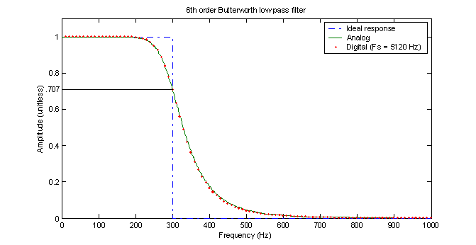
Figure 1 – Comparison of analog and digital Butterworth filters

To create the Butterworth digital filter, the MATLAB function ‘butter’ is used. According to the MATLAB documentation, this function uses a bilinear transformation with frequency prewarping to convert an analog prototype filter into a digital filter. This results in a transfer function in the frequency domain that is very consistent with the analog transfer function. Thus, at 300 Hz, the magnitude response of both filters is .70711, which is equivalent to -3.01 dB. The butter function uses prewarping at the cutoff frequency, which guarantees that the analog response and digital response will be the same at the cutoff frequency, which is exactly what is observed in figure 1.

To compare with a digital Chebyshev filter, the MATLAB function ‘cheby1’ is used with a pass-band ripple of 0.500 dB specified. This creates a Chebyshev type I filter, which is equiripple in the passband and monotonic in the stopband. A type II Chebyshev filter is monotonic in the passband an equiripple in the stopband and does not have as steep a response as the type I. As with the Butterworth filter, MATLAB uses a bilinear transformation of an analog prototype to obtain the same frequency response as the equivalent analog filter. Figure 2 compares the Chebyshev type I with the Butterworth.

Unlike the Butterworth filter, the 3 dB frequency of the Chebyshev is NOT the specified the cutoff frequency. Instead, the magnitude of the filter at the cutoff frequency is near the specified -0.5 dB point and the actual 3 dB frequency is at about 310 Hz. The Chebyshev filter, however, is much steeper near the cutoff frequency.

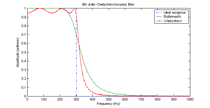
Figure 2 – Comparison of digital Chebyshev I and Butterworth filters

To create an elliptic filter, the MATLAB function ‘ellip’ function is used with a specified passband ripple of 0.500 dB and stopband attenuation of 40 dB. As with the others, MATLAB uses a bilinear transformation for the elliptic filter. The response is shown in figure 3 along with the other filters. From figure 3, it is clear that the elliptic filter has the steepest transition from the passband to the stopband and thus the 3 dB frequency is very close to 300 Hz. It also has a lower frequency ripple in the passband than the Chebyshev I filter.

To observe how the different filters perform in the time domain, the MATLAB function ‘filter’ is used in conjunction with a step input vector to produce figure 4.

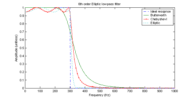
Figure 3 – Comparison of an elliptic filter with the others

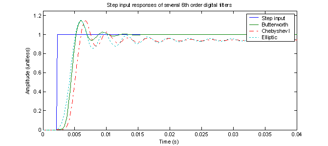
Figure 4 – Step responses of three digital filters

As expected the Butterworth filter settles to 1 while the other filters settle to approximately 0.95. This is expected because the Butterworth filter response in the frequency domain shows that it has a unity response at DC while the other filters have responses that are significantly less at f = 0 Hz. All three filters have similar overshoot of about 17% although the Butterworth filter settles much sooner than the others. This demonstrates that one cannot necessarily determine the ‘best’ filter by looking at the magnitude of the frequency response alone. If one could, one might assume from figure 3 that the elliptic filter is ‘best’ because it has the steepest transition. However, for the step input, the elliptic response has the most overshoot, the longest oscillation and it does not settle to the input value.

Part B – Infinite Impulse Response (IIR) Filters

In this part, the complete design of a second order digital Butterworth filter using the impulse invariance method is demonstrated without the aid of the MATLAB butter function. Starting with an analog filter and using a sampling frequency f_s = 320 Hz, the following checklist is used:

1. Get the analog transfer function G(s) of the analog filter.
2. Use the Laplace transform to convert the analog transfer function G(s) to the analog response in the time domain g(t).
3. Sample the analog response in the time domain by substituting nT for t where n is the sample number and T is the sample period 1/f_s. This results in h[n].
4. Take the Z-transform of h[n] to obtain H[z].

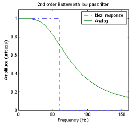Step 1 – Get the analog transfer function G(s) of the analog filter

Equation (1) is repeated to show the magnitude of the frequency response of a 2^nd order analog Butterworth filter.

What is needed, however, it not the magnitude of the frequency response |G(jω)|, but the frequency response G(jω).

Since j⁴ = 1, the j can be removed giving

. (2)

In order to complete the square under the root, add and subtract 2(ω/ω₀)²

. (3)

Rearranging,

. (4)

Now, consider that the magnitude of G(jω) is the magnitude of the numerator over the magnitude of the denominator.

(5)

Thus, by breaking the denominator into its conjugate roots, the magnitude is

, (6)

which means that the transfer function G(jω) is

, (7)

which is the same as

. (8)

Substituting s for jω and multiplying numerator and denominator by ω₀² gives

, (9)

which is now in a convenient form for taking the Laplace transform in step 2.

Step 2 – Convert G(s) to g(t) using the Laplace transform

To get the response in the time domain, the LaPlace transform is performed on (9) using the following transformation[1]:

Table 1 – Transformations for converting an analog filter to digital

Ha(s)	ha(t)	h[k]	H[z]

Solving for A, B, a, and c for the given function yields

. (10)

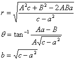
Solving for r, θ and b gives

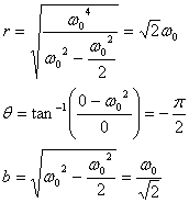(11)

The time domain response g(t) is left in terms of r, θ, and b temporarily for simplicity

(12)

Note that the T scaler is included in the table in anticipation of converting the continuous time function to a discrete time function. Since each sample in discrete time represents T amount of time, g(t) really represents the area under the curve for one sample period. In this manner CT and DT signals can be compared because the areas will be similar.

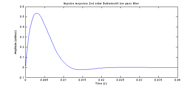
Figure 6 shows a plot of the analog impulse response.

Figure 6 – Impulse response of the analog Butterworth filter

Step 3 – Sample the time domain response g(t) to get the digital time domain response h[n]

Sampling is easily done by replacing t with nT and calling the result h[n].

(13)

The sampled points are illustrated in figure 7. The samples appear at every T (1/320 = .003125) s.

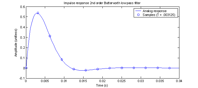
Figure 7 – Sampled impulse response

Step 4 – Perform the Z-transform

The Z-transform is performed using table 1.

. (14)

Multiplying both numerator and denominator by z^-2 gives

. (15)

This is a standard form for defining the transfer function H[z].

Now, substituting in r, θ, and b from (12), a from (11), and T= 1/320 will generate the a_i and b_i coefficients.

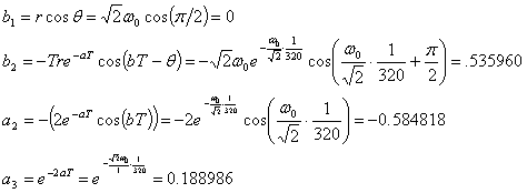(17)

Thus, the transfer function becomes

. (19)

The impinvar function in MATLAB can be used to perform steps 2 through 5 above to obtain the a and b coefficients. Listing 1 shows the results of the impinvar function. The MATLAB output agrees very well with the results obtained above.

Listing 1 – Demonstration of the impinvar function

Generating the response of the digital filter in the time domain is easily accomplished by rearranging the transfer function and taking the inverse Z-transform.

(20)

By cross multiplying

(21)

(22)

Now, take the inverse Z-transform to get

(23)

Equation (23) is used in MATLAB to ‘march’ through the sampled input points with a loop and create the digital step response shown in figure 9. If the impulse invariant method works as promised, then the impulse response obtained from equation (23) should match the samples from figure 7. Lo and behold, mach up exactly as shown in figure 8. The circles and squares line up very nicely.

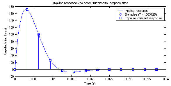
Figure 8 – Comparison of the analog response, samples and digital response

One might expect that, if the impulse response of the discrete time filter matches exactly with its analog counterpart, then the response of the discrete time filter of a different input function might also coincide with the analog response of the same input. Getting the response of the discrete time filter is easy using the same technique used to get the impulse response. Getting the analog response, however, is a different story.

There are two ways to see the response of the analog filter in the time domain. The impulse response g(t) can be convolved with the input function, or, the transfer function G(s) can be multiplied by the Laplace transform of the input function and then the inverse Laplace transform taken. For the unit step input, the following convolution table[2] is used to calculate the unit step response.

Table 2 – Convolution

f1(t)	f2(t)	f1(t)* f2(t)

The impulse response of the analog filter (12) is repeated (without the T scaler) here for reference

Using the convolution formula in table 2 gives

(24)

Figure 9 shows that the step responses of the two filters are NOT the same as is the case with the impulse responses

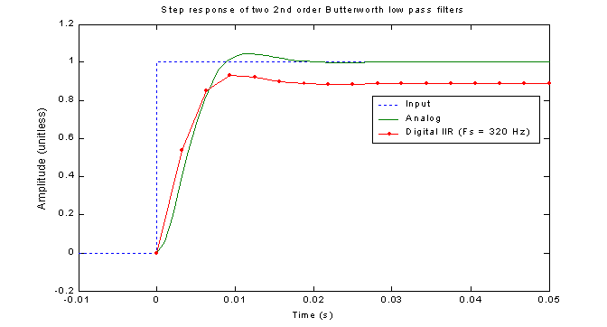
Figure 9 – Comparison of CT and DT step responses

The first thing that one might notice is that the steady state output of the digital filter is significantly attenuated. This fact begs one to ask, “What does the frequency response look like?” Figure 10 shows that the frequency response of the digital filter is much flatter than that of the analog filter and that at DC, there is significant attenuation, which agrees with what is seen in figure 9.

Although the responses are the same at the cutoff frequency, they differ by about 10% both at 0 Hz and at 160 Hz (the limit of the digital filter). This is significant attenuation in the pass-band and leakage in the stop-band. It indicates that this digital filter is probably not as good as its analog counterpart for most applications that would use a 2^nd order Butterworth filter. The advantage of using digital filters, however, is that it is simple to increase the order of the filter, while doing so in an analog system might prove difficult and/or expensive. Another interesting note is that the digital filter’s peak response is NOT at DC. It is, in fact, at around 20 Hz, which shows that the digital filter not only is a bit flattened, but that it also has a different shape than its analog counterpart.

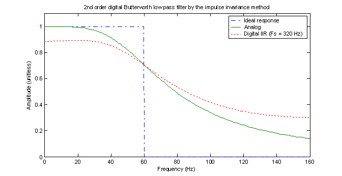
Figure 10 – Comparison of analog and digital Butterworth filters

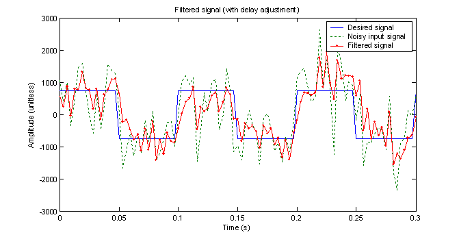
To observe the performance of this digital filter on a more realistic signal, a square wave is generated with white Gaussian noise added to it using the ‘randn’ function in MATLAB. To get the response of the noisy signal, the marching algorithm is used as before. Figure 11 shows the result of the filter compared with the noisy signal for 3 periods of the square wave. It is clear that the filter reduced many of the sharp peaks introduced by the noise. Some of this reduction is due to the filtering and some is due to the fact that this filter attenuates all frequencies by at least 10%.

To get some idea of how well the filter performs on the noisy signal, the SNR is taken of the input and output and compared. The following results were found for a simulation with 5000 samples:

Table 3 –Analysis of IIR filter

	% RMS error	SNR
Noisy input signal	100.3914 %	0.0781 dB
Filtered output signal	82.3673 %	3.8796 dB
Difference	82.3673 - 100.3914 = -18.0241 %	3.8796 - 0.0781 = 3.9578 dB

After running 10 such simulations, the SNR improvement averages out to about 3.8 dB. Your results may vary. Note that in order to get an accurate description of the error, the output has to be shifted ahead by one sample to account for the delay introduced by the filter. This assumes that we do not care about delay in the output, which is usually the case.

Figure 11 – Filtered signal

Part C – FIR filter design

In this section, an eighth-order, 60 Hz, Finite Infinite Response (FIR) low pass filter is designed using the Hamming window method. Similar to the impulse invariant method, the window method is used to design a filter that matches the impulse response of an analog filter at the sampled points. Unlike the impulse invariant method, however, the window method does not start with a realizable analog filter. Instead, an ideal filter is used to obtain the impulse response to be matched. The following steps are used to design the filter:

1. Choose an ideal analog filter

2. Find the impulse response of the ideal analog filter

3. Sample the impulse response N+1 times to create the b coefficients

Step 1 – Choose an ideal analog filter

The ideal filter to be used is the rectangular shape shown in figure 12. This represents the magnitude response of an ideal low pass filter with cutoff frequency of 60 Hz.

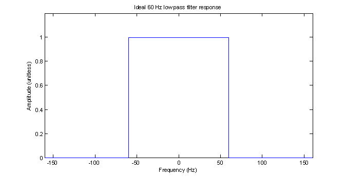
Figure 12 – Ideal low pass filter

Step 2 - Find the impulse response of the ideal analog filter

The magnitude of the response is not the complete description of filter’s response. There will most likely be some non-zero phase response over the frequency range as well. It turns out that letting the phase response be a linear function of frequency makes the design very simple[3]. Thus, the frequency response is defined by

(25)

The exponent term has two consequences, which are really two manifestations of the same thing. First, it results in a linear phase response in the frequency domain without affecting the magnitude. Second, it causes a delay of M terms in the impulse response of the filter, which can be seen in the following:

(26)

In order for the impulse response to be finite (i.e. Finite Impulse Response) and causal (i.e. cannot predict the future), (26) must be truncated so that it only represents a limited number of terms that are all greater than or equal to zero. This is illustrated in figure 13.

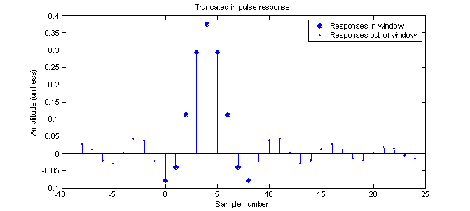
Figure 13 – Example of a windowed impulse response

Step 3 - Sample the impulse response N+1 times to create the b coefficients

By Limiting the number of terms to N+1, equation (26) becomes

(27)

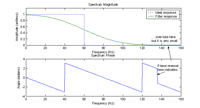
In figure 13, all points are a result of (26) while the large dots are a result of (27) only, making the response finite. By letting M= ½ N, the first large dot coincides with sample number 0 so the filter is now causal as well. Therefore, (27) represents the impulse response of a realizable FIR filter. The filter’s frequency response is shown in figure 14. The magnitude has a non-flat response in both the passband and stopband and there are side lobes in the stopband. As expected, the phase is linear (except for the reversals where the magnitude reaches 0). To implement the filter, the points represented by the big dots in figure 14 become the b coefficients for use in the marching equation or the MATLAB filter function.

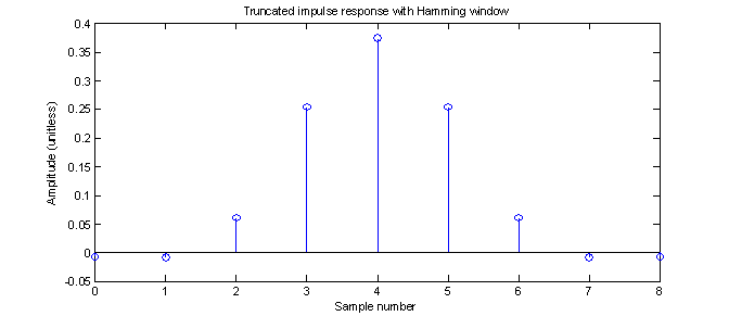
The filter represented by (27) can be improved by simply applying a non-rectangular window to the truncated points. A Hamming window works well for this purpose. Figure 15 shows the truncated impulse response after applying the Hamming window. Note that the first and last points have a magnitude of nearly zero. As was seen in exercise 1, this ‘smoothing’ of the sampling at the endpoints should result in fewer side lobes in the frequency response. Figure 16 shows the response of the windowed filter and it does indeed have reduced side lobes. In fact, they are almost completely gone.

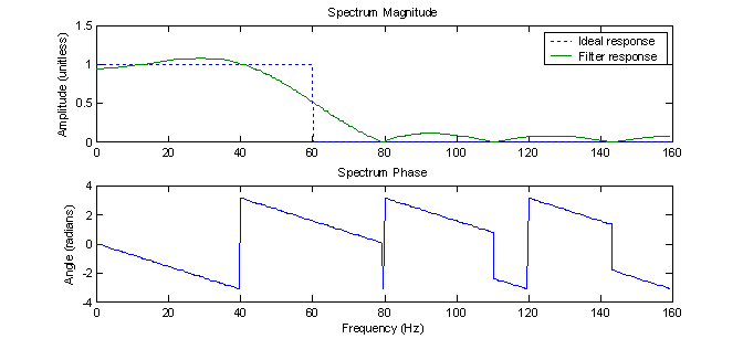
Figure 14 – Frequency response of 8^th order FIR filter with rectangular window

Figure 15 – Truncated impulse response of 8^th order FIR filter with Hamming window

Figure 16 – Frequency response of 8^th order FIR filter with Hamming window

Normally, one might want to test the new filter with an impulse input to verify its impulse response but for this filter, the impulse response defines the filter so that would be a trivial exercise. To test the FIR filter on a signal, as step function is applied, as was done in part B.

Figure 17 – Step response of a 8^th order FIR filter with Hamming window

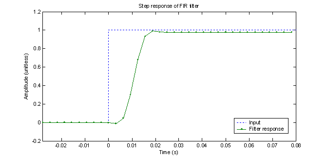
Figure 17 shows the step response of the FIR filter. It has a delay of N+1 samples before it gets to the steady state value, as expected. The DC steady state value is slightly under unity as is indicated by figure 16.

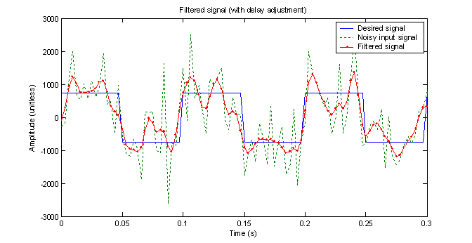
Once again, the noisy signal is applied to observe how the filter responds to a more realistic signal. The result is shown in figure 18. Just by observation, the filtered output seems to be smoother than that of the IIR filter in part B.

Figure 18 - Response of a 8^th order FIR filter with Hamming window on the noisy signal

To get a more quantitative description of the filter, the same type of analysis that was done in part B is performed for the FIR filter. The results are shown in table 4.

Table 4 –Analysis of FIR filter

	% RMS error	SNR
Noisy input signal	98.5067 %	0.3009 dB
Filtered output signal	55.6309 %	11.7286 dB
Difference	55.6309 - 98.5067 = -42.8757 %	11.7286 - 0.3009 = 11.4277 dB

As table 4 shows, the SNR improvement is around 11.4 dB, which is a significant improvement from the 2^nd order IIR filter from part B.

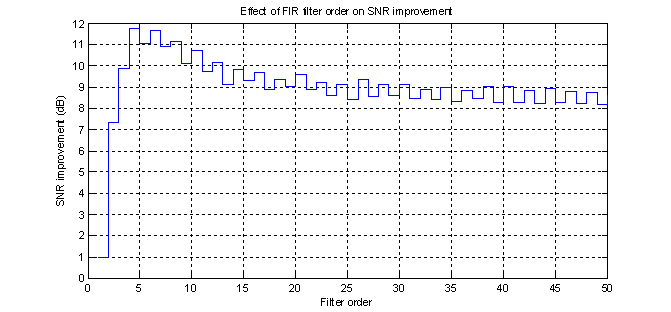
To explore the effect of changing the filter order on the SNR improvement, the FIR algorithm was made into a function with a MATLAB .m file. This function was then run with different values of N from 1 to 50 and the SNR improvement calculated. As expected, as the order went up, the SNR improvement also increased. What was not expected, however, was that once the filter order went over 4, which resulted in an SNR improvement of 11.75, the SNR improvement went down and seemed to approach an asymptote of about 8.5 dB. Another interesting phenomenon is that once the initial gains were realized with an order of 4 or more, the even order (6,8,10 etc.) filters consistently resulted in an SNR improvement about 0.5 dB over the odd ordered filters. These observations are illustrated in figure 19.

Figure 19 – Effect of N on the SNR improvement for the given noisy signal

Part D – Least Mean Squares adaptive filter

In this part, an 8^th order adaptive filter is designed and tested using the least mean square algorithm. This is an FIR filter whose b coefficients are changed on-the-fly for some period of time while it adapts to the input signal. The following function is used to change the b coefficients while the filter is adapting:

(28)

Where represents the new set of b coefficients, µ is a constant, N is the filter order, is the variance of the current set of input values, e_k is the error of the current sample with respect to the desired signal and is the set of inputs going back in time N samples.

To determine when the filter should stop adapting, the RMS of the most recent change in all of the b coefficients is compared with a constant (1%). If the RMS of the change between the new set of b coefficients and the old set is below 1%, then the algorithm figures that the coefficients are good and stops adapting. By trial and error, µ was set to 0.1, which seemed to provide reasonable results.

Due to the random nature of the noisy signal, every simulation yields a different result. In case shown in figure 20, the coefficients met the criteria after 88 samples and settled on a low pass type filter with maximum spectrum magnitude at about 20 Hz. The SNR analysis is shown in table 5.

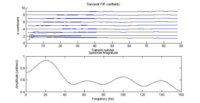
Figure 20 – Adapting coefficients and the final frequency response

Table 5 –Analysis of adaptive filter

	% RMS error	SNR
Noisy input signal	100.0642 %	-0.0128 dB
Filtered output signal	62.3460 %	9.4494 dB
Difference	62.3460 - 100.0642 = -37.7182 %	9.4494 – (-0.0128) = 9.4622 dB

This particular run had a SNR improvement of about 9.5 dB. After running many simulations it was found that the SNR improvement number varies widely. In some cases, it actually made the SNR improvement negative, indicating that it was adding more noise to the signal. Most simulations, however, had a SNR improvement between +5 dB and +10 dB.

The step response of the adaptive filter sometimes is very nice, and sometimes looks like figure 22. For this particular run, the DC gain is only about .72. One might think that this is not a good filter but one must remember that this filter was ‘trained’ on a 10 Hz square wave. It has never seen a plain old step response before. If a step response is the expected kind of signal, then the filter should be allowed to adapt to it. Sometimes, however, the filter adapts with a unity gain at DC and thus its step response is very nice.

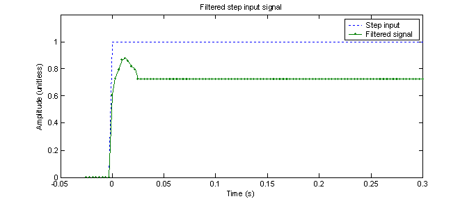
Figure 21 – Step response of 8^th order adaptive filter

Figure 22 shows the filter’s response to the same type of input signal that it was trained on.

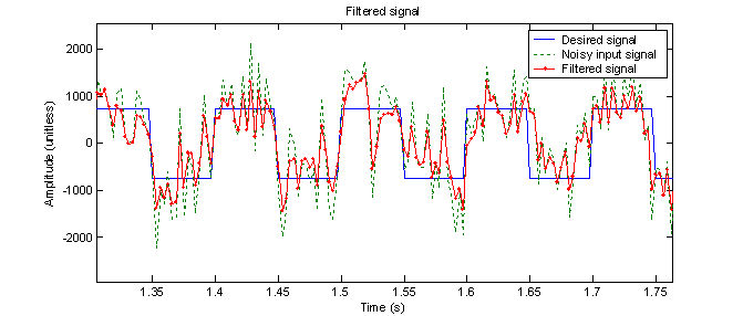
Figure 22 – 8^th order adaptive filter with noisy input signal

To see what is possible if the order is increased, it was increased by 10-fold to 80. Figures 23 and 24 show the results of one run on the noisy signal. Figure 23 demonstrates that the filter actually ‘learns’ the desired input signal. From Fourier series analysis, we know that a square wave has only odd harmonics. Thus, a 10 Hz, 50% duty cycle square has frequency components at 10 Hz, 30 Hz, 50 Hz etc. This is exactly what is seen in figure 23. For the N = 80 filter, almost every simulation yielded a similar result for the frequency response with peaks at the odd harmonics of 10 Hz.

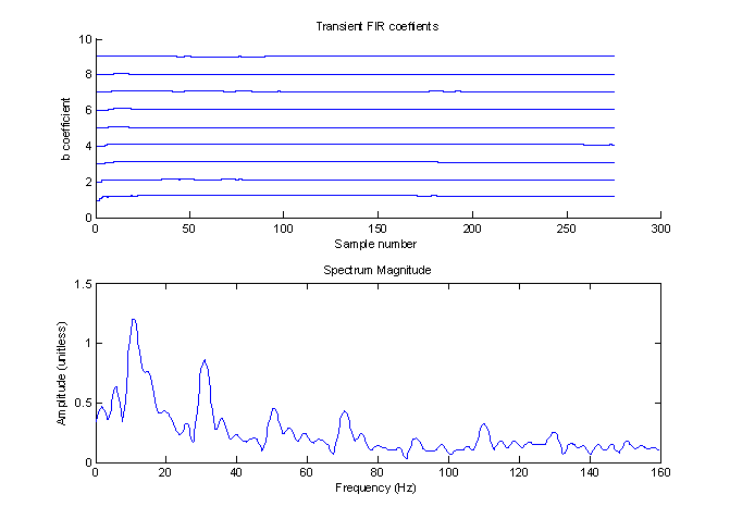
Figure 23 – Adapting coefficients and the final frequency response for N = 80

This filter resulted in an RMS improvement of 15.3 dB. The filter was also run with an order of 800, which resulted in an RMS improvement of 20.6 dB and is shown in figure 25.

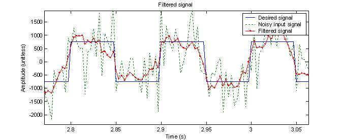
Figure 24 – 80^th order adaptive filter with noisy input signal

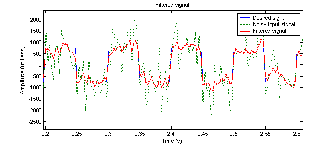
Figure 25 – 800^th order adaptive filter with noisy input signal (very nice)

Conclusions

Table 6 shows that of all the filters tested, the higher order adaptive filters proved best for the given noisy square wave signal. For the IIR filter, it seems that a 4^th order (and no higher) is best. This is a mystery to me but good news if I ever have to design an FIR filter with limited processing power.

Table 6 –Analysis of adaptive filter

Filter type	SNR Improvement of noisy signal
2^nd order IIR	3.8 dB
8^th order FIR	11.4 dB
4^th order FIR	11.7 dB
8^th order adaptive	9.4 dB
80^th order adaptive	15.3 dB
800^th order adaptive	20.6 dB

This project clearly demonstrated the steps to go through when designing a DSP filter and made it very clear exactly how to program a computer to do DSP filtering.

It was also shown that just because a digital filter looks good in the frequency domain doesn’t mean that it performs as well as one might expect on a particular signal in the time domain.

Appendix A – Code listing for entire project

% Kyle M. White

% EEE 233 Advanced DSP

% Exercise #2: Design of digital algorithms

clear;

% These are used in arrays to save vectors for final comparison

PartB = 1;

PartC = 2;

PartD = 3;

% =================================== PART A ==============================

Na = 6; % Order of the filter

Fo = 300; % Hz, the cutoff frequency

Wo = 2*pi*Fo;

Fs = 5120; % Hz, the sample frequency

Ws = 2*pi*Fs; % rad, the sample freq

T = 1/Fs;

% Create a vector for the ideal filter

fi = [0 299.99 300 1000];

Hi = [1 1 0 0];

% For comparison, show the transfer function of an analog filter

% Create the analog frequency vector

MaxFreq = 3*Fo;

Fa = 0:1:MaxFreq;

Wa = 2*pi*Fa;

HaButterworth = 1./(sqrt(1+(Wa/Wo).^(2*Na)));

MagHaButt = abs(HaButterworth);

% Digital

Samples = 512;

StepSize = 2*pi/Samples;

w=-pi:StepSize:pi-StepSize;

[b_butterworth,a_butterworth] = butter(Na,(2*Fo)/Fs);

hd = freqz(b_butterworth,a_butterworth,w);

Maghd = abs(hd);

% Plot the analog and digital Butterworth filters together

% Figure 1

plot(fi,Hi,'-.',Fa,MagHaButt,'-',Fs*w/(2*pi),Maghd,'.');

Xlim([0 1000]);

Ylim([0 1.1]);

Xlabel('Frequency (Hz)');

Ylabel('Amplitude (unitless)');

title('6th order Butterworth low pass filter');

legend('Ideal response','Analog','Digital (Fs = 5120 Hz)');

% Create the Chebyshev digital filter

[b_chebyshev,a_chebyshev] = cheby1(Na,0.5,(2*Fo)/Fs);

hdChebyshev = freqz(b_chebyshev,a_chebyshev,w);

% Plot the Chebyshev digital filter

% Figure 2

plot(fi,Hi,'-.',Fa,abs(HaButterworth),'-',Fs*w/(2*pi),abs(hdChebyshev),'.-');

Xlim([0 1000]);

Xlabel('Frequency (Hz)');

Ylabel('Amplitude (unitless)');

title('6th order Chebyshev low pass filter');

legend('Ideal resopnse','Butterworth','Chebyshev I');

% Create the Elliptic digital filter

[b_elliptic,a_elliptic] = ellip(Na,0.5,40,(2*Fo)/Fs);

hdElliptic = freqz(b_elliptic,a_elliptic,w);

% Plot the Elliptic digital filter

% Figure 3

plot(fi,Hi,'-.',Fa,abs(HaButterworth),'-',Fs*w/(2*pi),abs(hdChebyshev),'.-',Fs*w/(2*pi),abs(hdElliptic),':');

%plot(fi,Hi,'-.',Fa,abs(HaButterworth),'-',Fs*w/(2*pi),abs(hdElliptic),'.');

Xlim([0 1000]);

Xlabel('Frequency (Hz)');

Ylabel('Amplitude (unitless)');

title('6th order Elliptic low pass filter');

legend('Ideal resopnse','Butterworth','Chebyshev I','Elliptic');

% Apply the filters to a step input

% Figure 4

Samples = 512;

StepSize = 1/Fs;

t = 0:StepSize:StepSize*(Samples-1);

X = zeros(256,1);

X = cat(1,zeros(12,1),ones(500,1));

%X = ones(512,1);

y_butterworth = filter(b_butterworth,a_butterworth,X);

y_chebyshev = filter(b_chebyshev,a_chebyshev,X);

y_elliptic = filter(b_elliptic,a_elliptic,X);

plot(t,X,'-',t,y_butterworth,'-',t,y_chebyshev,'-.',t,y_elliptic,':');

legend('Step input','Butterworth','Chebyshev I','Elliptic');

title('Step input responses of several 6th order digital filters');

Ylim([0 1.25]);

Xlim([0 0.04]);

% =================================== PART B ==============================

% Create the input signal

clear;

Nb = 2;

Fs = 320; % Hz, the samle frequency

T = 1/Fs;

% Create a 2nd order analog Butterworth filter

% with cutoff of 60 Hz

hold off;

Fo = 60; % Hz

Wo = 2*pi*Fo; % radians

% The ideal response

Fi = [0 Fo-.00001 Fo+.00001 Fs];

Hi = [1 1 0 0];

% The analog frequency response

MaxFreq = 3*Fo;

Fa = 0:1:MaxFreq;

Wa = 2*pi*Fa;

HaButterworth = 1./(sqrt(1+(Wa/Wo).^(2*Nb)));

MagHaButt = abs(HaButterworth);

% The digital frequency response (Listing 1 in the report)

Fo = 60; % Hz

Wo = 2*pi*Fo; % radians

b=[Wo^2];

a=[1 Wo*sqrt(2) Wo^2];

[bz,az]=impinvar(b,a,320);

bz;

az;

% This works too

[HaButterworth,wana] = freqs(b,a);

% ========================== PART B Frequency response =========================

% Compare the frequency response of th IIR and analog filters

[H,w]=freqz(bz,az);

f = (160/pi).*w';

% Show just the analog frequency response

% Figure 5

plot(Fi,Hi,'-.',wana/(2*pi),abs(HaButterworth),'-');

Xlim([0 Fs/2]);

Ylim([0 1.1]);

Xlabel('Frequency (Hz)');

Ylabel('Amplitude (unitless)');

title('2nd order Butterworth low pass filter');

legend('Ideal response','Analog');

% Show the impulse response of the analog filter

% Figure 6

maxt = .04;

ta = 0:maxt/100:maxt;

Wo = 2*pi*60;

r = sqrt(2)*Wo;

a = Wo/sqrt(2);

b = a;

theta = -pi/2;

goft = T*r*exp(-a*ta).*cos(b.*ta + theta); % Equation (12)

plot(ta,goft);

Xlabel('Time (s)');

Ylabel('Amplitude (unitless)');

title('Impulse response 2nd order Butterworth low pass filter');

% Sample the impulse response of the analog filter

% Figure 7

hold on; % save the previous plot

T = 1/Fs;

nT = 0:T:maxt;

gofnT = T*r*exp(-a*nT).*cos(b.*nT + theta); % Equation (12)

plot(nT,gofnT,'o');

legend('Analog response','Samples (T = .003125)');

% Compare the analog and digital impulse responses

nT = 0:T:.05;

% Create the digital impulse function

xofn = zeros(size(nT));

xofn(1) = 1/T;

% ----------- From here....

% Append 2 zeros to the beginning of the x an y arrays

xofn = [0 0 xofn];

yofn = [0 0];

for n = 3:1:size(nT,2); % start with 3 cuz that the first 'real' element in the array

yofn(n) = bz(2)*xofn(n-1) - az(2)*yofn(n-1) - az(3)*yofn(n-2); % Equation (23)

end

% Now remove the 2 zeros that were added

yofn = yofn(3:size(nT,2));

xofn = xofn(3:size(nT,2));

% ------------ .... to here is what the 'filter' function does for the given

% as, bs and input x

yofnfilt = filter(bz,az,xofn);

% Plot the impulse response of the analog, sampled, and digital

% Figure 8

hold on; % Save the last plot

stem(nT(1:size(nT,2)-2),yofn,'s');

%plot(nT(1:size(nT,2)-2),yofnfilt,'x'); % Just used to verify the filter function. It works

legend('Analog response','Samples (T = .003125)','Impulse Invariant response');

Xlim([0 0.04]);

hold off;

% ========================== PART B Step response =========================

% Plot the step response of the analog filter and digital filter

% Compare the step response of the IIR and analog filters

% Ideal

ti = [-.01 0-.00001 0+.00001 1];

IdealResponse = [0 0 1 1];

% Analog

t1=0:.001:.1;

goft = 1 -sqrt(2)*(exp((-Wo/sqrt(2))*t1)).*cos((Wo/sqrt(2))*t1 - (pi/4)); % Equation (24)

% Digital - use marching equation

nT = 0:T:.05;

xofn = ones(size(nT));

% Append 2 zeros to the beginning of the x an y arrays

xofn = [0 0 xofn];

yofn = [0 0];

for n = 3:1:size(nT,2); % start with 3 cuz that is the first 'real' element in the array

yofn(n) = bz(2)*xofn(n-1) - az(2)*yofn(n-1) - az(3)*yofn(n-2); % Equation (23)

end

% Now remove the 2 zeros that were added

yofn = yofn(3:size(nT,2));

xofn = xofn(3:size(nT,2));

plot(ti,IdealResponse,':',t1,goft,'-',nT(1:size(nT,2)-2),yofn,'.-');

Xlim([-0.01 .05]);

Xlabel('Time (s)');

Ylabel('Amplitude (unitless)');

title('Step response of two 2nd order Butterworth low pass filters');

legend('Input','Analog','Digital IIR (Fs = 320 Hz)');

% Compare analog and digital responses

% Figure 10

MagDigFilter = abs(H');

plot(Fi,Hi,'-.',wana/(2*pi),abs(HaButterworth),'-',f,MagDigFilter,':');

Xlim([0 Fs/2]);

Ylim([0 1.1]);

Xlabel('Frequency (Hz)');

Ylabel('Amplitude (unitless)');

title('2nd order digital Butterworth low pass filter by the impulse invariance method');

legend('Ideal response','Analog','Digital IIR (Fs = 320 Hz)');

% Do the same thing with a noisy signal

Fp = 10; % Hz, frequency of the square wave

Samples = 5000;

% t = 0:T:Samples*T;

% s = 750*square(2*pi*Fp*t);

% noise = 750*randn(size(t,2),1); % Normalized white Gaussian noise

% noise = noise';

% NoisySig = s+noise;

tsignal = 0:T:Samples*T;

s = 750*square(2*pi*Fp*tsignal);

sPadded = [zeros(1,Nb) s];

noise = 750*randn(1,length(tsignal)); % Normalized white Gaussian noise

noisePadded = [zeros(1,Nb) noise];

NoisySig = s+noise;

NoisySigPadded = sPadded+noisePadded;

t = -Nb*T:T:-T;

t = [t tsignal];

plot(t,sPadded,t,NoisySigPadded,'.'); % Check plot

subplot(1,1,1);

% Setup the input function and initial conditions

xofn = NoisySigPadded;

yofn = zeros(1,Nb+1);

LengthOfAzMinusOne = length(az)-1;

LengthOfBzMinusOne = length(bz)-1;

az(1) = 0;

for n = Nb+1:1:Samples+Nb+1; % start with N+1 cuz that is the first 'real' element in the array

yofn(n) = 0; % Increase the size of the y array

yArrForAs = fliplr(yofn(n-LengthOfAzMinusOne:n-1)); % Create a flipped array for x

xArrForBs = fliplr(xofn(n-LengthOfBzMinusOne:n)); % Create a flipped array for y

% Run the filter for one sample

yofn(n) = sum(bz.*xArrForBs) - sum(az(1:LengthOfAzMinusOne).*yArrForAs); % Equation (23)

end

% for n = 3:1:size(nT,2); % start with 3 cuz that the first 'real' element in the array

% yofn(n) = bz(2)*xofn(n-1) - az(2)*yofn(n-1) - az(3)*yofn(n-2); % Equation (23)

% end

% Adjust for the delay

yofnshift = circshift(yofn,[0 -1]);

% Figure 11

plot(t,sPadded,'-',t,xofn,':',t,yofnshift,'.-');

Xlim([0 .3]);

Xlabel('Time (s)');

Ylabel('Amplitude (unitless)');

title('Filtered signal (with delay adjustment)');

legend('Desired signal','Noisy input signal','Filtered signal');

% Error analysis

Sig_RMS = sqrt(sum(s.^2)/length(s)); % Test RMS calculation - should be 750

InputErr_RMS = sqrt(sum((noise).^2)/length(noise));

InputPercentRMSError = 100*(InputErr_RMS/Sig_RMS)

ErrAnalysis(1,1) = InputPercentRMSError;

InputSNR = 20*log(Sig_RMS/InputErr_RMS);

ErrAnalysis(1,2) = InputSNR;

OutputErr_RMS = sqrt(sum((yofnshift(3:end)-s).^2)/length(s));

OutputPercentRMSError = 100*(OutputErr_RMS/Sig_RMS);

ErrAnalysis(2,1) = OutputPercentRMSError;

OutputSNR = 20*log(Sig_RMS/OutputErr_RMS);

ErrAnalysis(2,2) = OutputSNR;

SNR_Improvement = OutputSNR - InputSNR;

ErrAnalysis(3,1) = InputPercentRMSError - OutputPercentRMSError;

ErrAnalysis(3,2) = SNR_Improvement;

disp(ErrAnalysis);

% ======================== PART C - Ideal filter ==============================

clear;

Fs = 320;

T = 1/Fs;

% Show the ideal filter

Nc = 8;

LittleBit = 1e-5;

Fc = 60;

Fs = 320; % Sample frequency

fLim = Fs/2;

wi = [-fLim -Fc-LittleBit -Fc+LittleBit Fc-LittleBit Fc+LittleBit fLim];

Hi = [0 0 1 1 0 0];

% Figure 13

plot(wi,Hi);

Xlim([-fLim fLim]);

Ylim([0 1.2]);

Xlabel('Frequency (Hz)');

Ylabel('Amplitude (unitless)');

title('Ideal 60 Hz low pass filter response');

% Show the truncated inverse DT transform

M = Nc/2;

Wc = 2*pi*Fc;

Wcn = (2*Fc)/Fs; % Normailzed cutoff frequency

WcnOverPi = Wcn/pi;

n=0:Nc;

hofn = (Wcn)*ksinc(pi*Wcn*(n-M));

%plot(n,hofn,'o','MarkerFaceColor','b');

%hold on;

n1=-Nc:3*Nc;

hofn1 = (Wcn)*ksinc(pi*Wcn*(n1-M));

% Figure 14

plot(n,hofn,'ob',n1,hofn1,'.','MarkerFaceColor','b');

hLabel = Xlabel('Sample number');

Ylabel('Amplitude (unitless)');

title('Truncated impulse response');

Legend('Responses in window','Responses out of window');

hold on;

stem(n1,hofn1,'.');

% Compare with fir1 function

win = ones(Nc+1,1)';

b=fir1(Nc,Wcn,win,'noscale');

stem(n,b,'s');

% ======================== PART C - FIR filter ==============================

% Show the frequency response with a rectangular windwow

[H,w]=freqz(hofn,1);

w = (Fs/(2*pi))*w;

subplot(2,1,1);

% Figure 15

plot(wi,Hi,':',w,abs(H),'-');

title('Spectrum Magnitude');

Ylabel('Amplitude (unitless)');

Legend('Ideal response','Filter response');

Xlim([0 Fs/2]);

subplot(2,1,2);

plot(w,angle(H));

Xlabel('Frequency (Hz)');

Ylabel('Angle (radians)');

title('Spectrum Phase');

% Compare with fir1 function

subplot(2,1,1);

[Hb,wb]=freqz(b,1);

wb = (Fs/(2*pi))*wb;

plot(w,abs(H),'-',wb,abs(Hb),'-')

% Do the same but with a Hamming window

subplot(1,1,1);

win = 0.54-(0.46.*cos(2*pi.*n./Nc));

hham = hofn.*win;

% Figure 16

stem(n,hham);

hLabel = Xlabel('Sample number');

Ylabel('Amplitude (unitless)');

title('Truncated impulse response with Hamming window');

[Hham,w] = freqz(hham,1);

w = (Fs/(2*pi))*w;

% Figure 17

% Magnitude

subplot(2,1,1);

plot(wi,Hi,':',w,abs(Hham),'-');

Xlim([0 Fs/2]);

Ylim([0 1.2]);

Xlabel('Frequency (Hz)');

Ylabel('Amplitude (unitless)');

title('Spectrum Magnitude');

Legend('Ideal response','Filter response');

% Phase

subplot(2,1,2);

plot(w,angle(Hham),'-');

Xlim([0 Fs/2]);

Xlabel('Frequency (Hz)');

Ylabel('Angle (radians)');

title('Spectrum Phase');

%Compare with the fir1 function

bham = fir1(Nc,Wcn,'noscale');

[Hbham,wb] = freqz(bham,1);

wb = (Fs/(2*pi))*wb;

plot(w,abs(Hham),'-',w,abs(Hbham),'-');

% ======================= PART C - marching ==============================

% OK, now the bs are in bham, use the marching algorithm

% Plot the step response of the analog filter and digital filter

% Compare the step response of the FIR and analog filters

% Ideal

ti = [-1 0-LittleBit 0+LittleBit 1];

IdealResponse = [0 0 1 1];

% Digital - use marching equation

nT = -(Nc+1)*T:T:Nc/100; % N/100 results in a nice sample for any N

% Setup the input function and initial conditions

xofn = [zeros(1,Nc+1) ones(1,length(nT) - (Nc+1))];

yofn = zeros(1,Nc+1);

for n = Nc+2:1:length(nT); % start with N+2 cuz that is the first 'real' element in the array

yofn(n) = 0;

for i = 0:1:length(bham)-1

yofn(n) = yofn(n) + bham(i+1)*xofn(n-i);

end

end

yfilt = filter(bham,1,xofn); % For comparison

% Figure 18

subplot(1,1,1);

plot(ti,IdealResponse,':',nT,yofn,'.-') %,'.-',nT,yfilt);

Xlim([-(Nc+1)*T Nc/100]);

Xlabel('Time (s)');

Ylabel('Amplitude (unitless)');

title('Step response of FIR filter');

legend('Input','Filter response');

% =========================== PART C - Noisy signal ==============================

% Do the same thing with a noisy signal

Fp = 10; % Hz, frequency of the square wave

Samples = 5000; % Number of samples will be Samples + 1 + Nc

tsignal = 0:T:Samples*T;

s = 750*square(2*pi*Fp*tsignal);

s = [zeros(1,Nc) s];

noise = 750*randn(1,length(tsignal)); % Normalized white Gaussian noise

noise = [zeros(1,Nc) noise];

NoisySig = s+noise;

t = -Nc*T:T:-T;

t = [t tsignal];

plot(t,s,t,NoisySig);

% Filter noisy signal

% nT = -(Nc)*T:T:length(s)*T; % N/100 results in a nice sample for any N

% Setup the input function and initial conditions

xofn = NoisySig;

yofn = zeros(1,Nc+1);

for n = Nc+1:1:Samples+Nc+1; % start with N+2 cuz that is the first 'real' element in the array

% Create a flipped array for x

% NOTE: Don't really need to do it this way for THIS filter

% because bham is symmetrical anyway.

xarr = fliplr(xofn(n-Nc:n));

% Run the filter for one sample

yofn(n) = sum(bham.*xarr);

end

% Test plot

plot(t,s,'-',t,xofn,':',t,yofn,'.-');

% Shift the output so it lines up with the input (and keeps the number of

% points the same)

yofnshift = circshift(yofn,[0 floor(-Nc/2)]);

% Figure 19

plot(t,s,'-',t,xofn,':',t,yofnshift,'.-');

Xlabel('Time (s)');

Ylabel('Amplitude (unitless)');

title('Filtered signal (with delay adjustment)');

legend('Desired signal','Noisy input signal','Filtered signal');

% Filter analysis

Sig_RMS = sqrt(sum(s.^2)/length(s)); % Test RMS calculation - should be 750

InputErr_RMS = sqrt(sum((noise).^2)/length(noise));

InputPercentRMSError = 100*(InputErr_RMS/Sig_RMS);

ErrAnalysis(1,1) = InputPercentRMSError;

InputSNR = 20*log(Sig_RMS/InputErr_RMS);

ErrAnalysis(1,2) = InputSNR;

OutputErr_RMS = sqrt(sum((yofnshift(Nc+1:end - floor(Nc/2))-s(Nc+1:end - floor(Nc/2))).^2)/length(s));

OutputPercentRMSError = 100*(OutputErr_RMS/Sig_RMS);

ErrAnalysis(2,1) = OutputPercentRMSError;

OutputSNR = 20*log(Sig_RMS/OutputErr_RMS);

ErrAnalysis(2,2) = OutputSNR;

SNR_Improvement = OutputSNR - InputSNR;

ErrAnalysis(3,1) = InputPercentRMSError - OutputPercentRMSError;

ErrAnalysis(3,2) = SNR_Improvement;

disp(ErrAnalysis);

% =================================== Still PART C ==============================

% Figure 12

Xlim([0 .3]);

Xlabel('Time (s)');

Ylabel('Amplitude (unitless)');

title('Filtered signal (with delay adjustment)');

legend('Desired signal','Noisy input signal','Filtered signal');

% ===================== Find point of diminishing returns =====================

if 0

for N = 1:50;

ErrAnal = FIRfunction(N,320,0);

SNRs(N) = ErrAnal(3,2);

end

stairs(SNRs);

Xlabel('Filter order');

Ylabel('SNR improvement (dB)');

title('Effect of FIR filter order on SNR improvement');

grid on;

end

% =================================== PART D ==============================

clear Nc;

% Least squares adaptive filter

% start with the bs from part c

Nd = 800;

badapt = zeros(1,Nd+1);

mu = 0.1;

TwoMu = 2*mu;

Fp = 10; % Hz, frequency of the square wave

Samples = 5000; % Number of samples will be Samples + 1 + Nc

tsignal = 0:T:Samples*T;

s = 750*square(2*pi*Fp*tsignal);

s = [zeros(1,Nd) s];

noise = 750*randn(1,length(tsignal)); % Normalized white Gaussian noise

noise = [zeros(1,Nd) noise];

NoisySig = s+noise;

t = -Nd*T:T:-T;

t = [t tsignal];

plot(t,s,t,NoisySig);

% Setup the input function and initial conditions

xofn = NoisySig;

yofn = zeros(1,Nd);

% Let it run until the Bs don't change much

fAdapt = 1;

%Shift = ceil(1.5*Nd)+1;

AdaptRound = 1;

while fAdapt

for n = Nd+1:1:Samples+Nd+1;

Xk = fliplr(xofn(n-Nd:n)); % Create the X array

yofn(n) = sum(badapt.*Xk); % Find the next y value

Err = s(n) - yofn(n); % Get the error term

NSigmaSquared = Nd*sum(Xk.^2)/length(Xk); % N times sigma squared

TwoMuOverNSigmaSquared = TwoMu/NSigmaSquared;

% Save the bs

for bi = 1:Nd+1;

SavedBs(bi,AdaptRound) = badapt(bi);

if AdaptRound > 1

DeltaBs(bi) = SavedBs(bi,AdaptRound) - SavedBs(bi,AdaptRound - 1);

end

end

% Change all the Bs at one time using arrays

badapt = badapt + (TwoMuOverNSigmaSquared*Err)*Xk; % Equation (28)

if AdaptRound > 1

ChangeOfBs = DeltaBs./badapt;

RMSChangeOfBs = sqrt((sum(ChangeOfBs.^2))/length(ChangeOfBs));

if RMSChangeOfBs < 0.01

fAdapt = 0

break

end

end

AdaptRound = AdaptRound+1;

end

end

% Test plot

%plot(t,s,'-',t,xofn,':',t(1:length(yofn)),yofn,'.-');

% Show the results of the adaptation

% Figure 21

figure(1);

%subplot(3,1,1);

%plot(t,s,'-',t,xofn,'-',t(1:length(yofn)),yofn,'.-') %,'.-',nT,yfiltyofnForPlotting;

%Xlim([0 0.5]);

[Hadapt,wadapt] = freqz(badapt,1);

fadapt = (Fs/2)*(wadapt/pi);

subplot(2,1,2);

plot(fadapt,abs(Hadapt));

Xlim([0 Fs/2]);

Xlabel('Frequency (Hz)');

Ylabel('Amplitude (unitless)');

title('Spectrum Magnitude');

subplot(2,1,1);

PlotArr(1,1) = 0;

for bi = 1:min(9,length(badapt)); % Only do up to 9 of the bs

hold on;

PlotArr = SavedBs(bi,1:end);

PlotArr = PlotArr + (bi/1)*ones(1,length(PlotArr));

stairs(PlotArr);

end

Xlabel('Sample number');

Ylabel('b coefficient');

title('Transient FIR coeffients');

hold off;

% Now run the step signal through

% Figure 22

StepInput = [zeros(1,Nd) ones(1,length(tsignal))];

for n = Nd+1:1:Samples+Nd+1;

Xk = fliplr(StepInput(n-Nd:n));

yofn(n) = sum(badapt.*Xk);

end

figure(2);

subplot(1,1,1);

plot(t,StepInput,':',t,yofn,'.-');

Xlabel('Time (s)');

Ylabel('Amplitude (unitless)');

Ylim([0 1.2]);

Xlim([-0.05 0.3]);

title('Filtered step input signal');

legend('Step input','Filtered signal');

% Now run the whole noisy signal through

for n = Nd+1:1:Samples+Nd+1;

Xk = fliplr(xofn(n-Nd:n));

yofn(n) = sum(badapt.*Xk);

end

figure(2);

% Figure 23

subplot(1,1,1);

plot(t,s,'-',t,xofn,':',t,yofn,'.-');

Xlabel('Time (s)');

Ylabel('Amplitude (unitless)');

title('Filtered signal');

legend('Desired signal','Noisy input signal','Filtered signal');

% Filter analysis

Sig_RMS = sqrt(sum(s.^2)/length(s)); % Test RMS calculation - should be 750

InputErr_RMS = sqrt(sum((noise).^2)/length(noise));

InputPercentRMSError = 100*(InputErr_RMS/Sig_RMS);

ErrAnalysis(1,1) = InputPercentRMSError;

InputSNR = 20*log(Sig_RMS/InputErr_RMS);

ErrAnalysis(1,2) = InputSNR;

OutputErr_RMS = sqrt(sum((yofn(Nd+1:end - floor(Nd/2))-s(Nd+1:end - floor(Nd/2))).^2)/length(s));

OutputPercentRMSError = 100*(OutputErr_RMS/Sig_RMS);

ErrAnalysis(2,1) = OutputPercentRMSError;

OutputSNR = 20*log(Sig_RMS/OutputErr_RMS);

ErrAnalysis(2,2) = OutputSNR;

SNR_Improvement = OutputSNR - InputSNR;

ErrAnalysis(3,1) = InputPercentRMSError - OutputPercentRMSError;

ErrAnalysis(3,2) = SNR_Improvement;

disp(ErrAnalysis);

---

[1] Lathi, B.P., Signal Processing & Linear Systems, Berkeley-Cambridge Press, Carmichael, CA, 1998, p 736

[2] Lathi, B.P., Signal Processing & Linear Systems, Berkeley-Cambridge Press, Carmichael, CA, 1998, p 125

[3] Chen, Chi-Tsong, Digital Signal Processing, Oxford University Press, Oxford, NY. p. 305